
Abstract
The HIsarna process is a new and breakthrough smelting reduction process for hot metal (liquid iron) production from iron ores and coal directly fed into the reactor. The flue gas from the main reactor enters the off-gas system containing small amounts of H2, CO and carbon particles which need to be removed before further treatment by post combustion oxygen injection. A three-dimensional Computational Fluid Dynamics (CFD) simulation of the HIsarna off-gas system is performed and validated using a detailed reaction mechanism and kinetic data for post-combustion of a CO–H2 mixture and carbon particles. Using the validated model, a series of simulations were performed to investigate the effect of water quenching and post combustion oxygen injection. It was found that water quenching can significantly reduce the off-gas temperature. It is also possible to reduce oxygen injection during operations where inlet CO content of the off-gas system is low.
Introduction
The HIsarna process is a new and breakthrough smelting reduction technology for the production of liquid hot metal from iron ores and coal directly fed into the reactor. In comparison with the blast furnace route, coking and iron ore agglomeration (sintering and pelletizing) processes are eliminated which inherently leads to about a 20% reduction in CO2 emission. This reduction can be further increased, up to 80–90%, by incorporating carbon capture and storage (CCS) technologies.
The process is a combination of the Cyclone Converter Furnace (CCF) technology and the HIsmelt technology (which was developed by RioTinto [1]) built in pilot scale, capable of producing 8 ton/hr hot metal in the IJmuiden Works of Tata Steel Europe in 2010 and since that time it has been under development towards industrial demonstration.
The main reactor, off-gas system and other downstream components are shown in Figure 1. The main reactor can be divided into two sections. Fine iron ore is injected into the CCF along with pure oxygen. The oxygen is needed as an oxidizer to partly combust the CO–H2 compound of the off-gasses coming from the Smelting Reduction Vessel (SRV). The combustion process provides heat to pre-reduce and melt the iron ore during the flight time and ultimately is deposited against the wall of the furnace. The accumulation of the particles on the wall creates a liquid film to drip along the wall and fall into the molten iron bath of the SRV. The outlet gas from CCF mainly is a mixture of CO2–H2O–N2 with a small amount of CO, H2, O2 and carbon particles. Schematic overview of the HIsarna pilot reactor, including its off-gas system.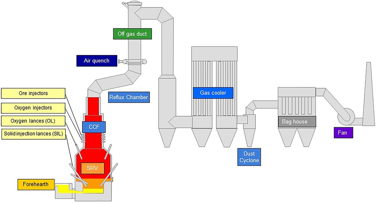
Coal is injected into the slag layer using a carrier gas and will partially penetrate the metal bath to carburize the molten iron. The coal particles in the slag will reduce pre-reduced iron oxide (FeO x ) droplets pouring into the bath from the CCF above. CO gas will be generated in the form of bubbles and will reach the top space of the SRV to combust with oxygen injected through oxygen lances (OL), providing the necessary heat in the SRV. The melt is separated into two molten layers, a top layer of slag and a bottom layer of molten hot metal. Both layers can be tapped individually, and the hot metal will be used for steelmaking.
Above the CCF there is an important section called the reflux chamber, which is a slightly angled horizontal pipe with two bends to treat the furnace off-gas by combusting any remaining CO, H2 and carbon particles. Above the reflux chamber the flue gas is quenched by injecting air or recycled off-gas. Downstream there will be additional water spray injection for further cooling. A schematic description of the off-gas system is presented in Figure 2. Off-gas system components and data acquisition points (point A: reflux chamber outlet, Point B: end of up leg, Point C: 3 m above water quench atomizers, Point D: exit to gas cooler).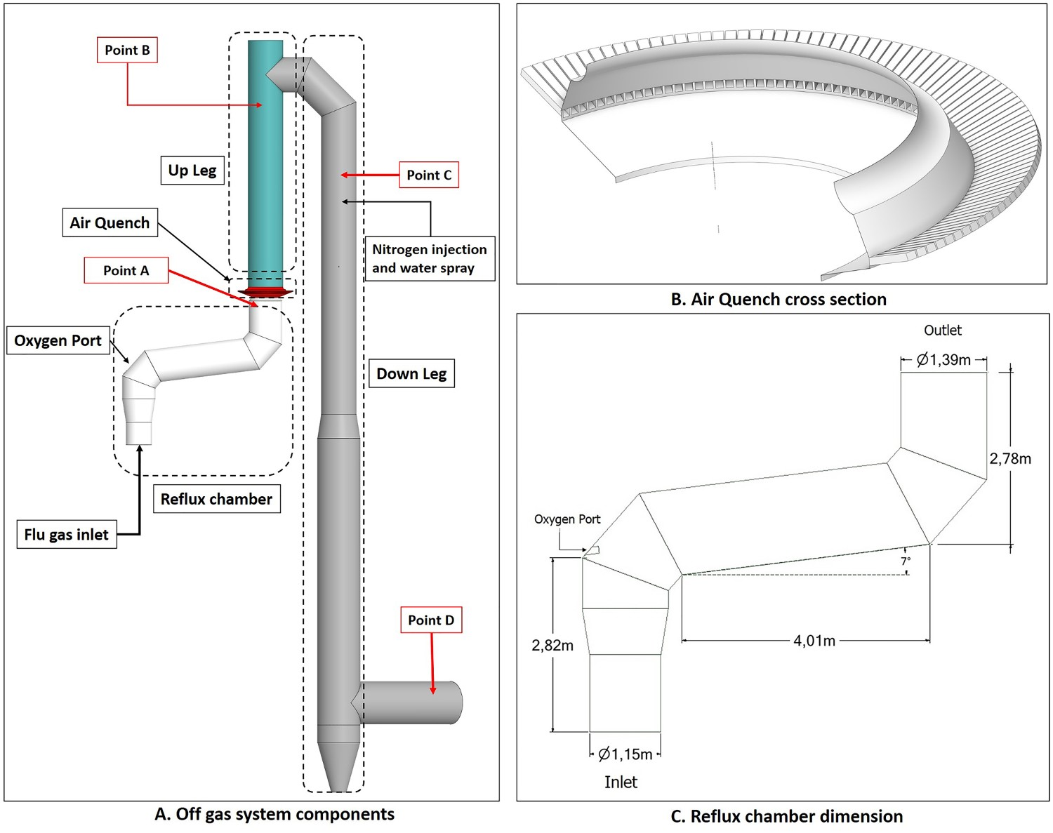
In this study, a model is developed to predict the behaviour of post-combustion of CO, H2 and carbon particles in the off-gas system. The model is validated using plant data and is used to investigate the effect of oxygen on the post-combustion to see if it is possible to reduce or optimize the oxygen injection flowrate. Furthermore, the effect of evaporative cooling for further temperature reduction is discussed to reach a proper temperature at the outlet of the off-gas system.
The most important factor in this study is to predict the combustion behaviour of the gaseous mixture correctly. To fulfil that a proper reaction mechanism and kinetic data is required. There have been numerous studies on reaction mechanisms, development of a kinetic database and numerical simulations of CO and H2 combustion.
Fotache et al. [2] have performed non-premixed simulation of a counter-current flowing CO–H2–N2 dry mixture with heated air jets using a detailed kinetic mechanism to investigate the effect of hydrogen on ignition regime. Dagaut et al. [3] have investigated the effect of NO and SO2 on the oxidation of a CO–H2 dry mixture in a jet-stirred reactor at atmospheric pressure with variable temperature (800–1400 K) and for various air equivalence ratios and initial concentrations of NO and SO2 (0 and 5000 ppm). Kim et al. [4] performed a numerical simulation of moist carbon monoxide oxidation for different pressures from 1 to 9.6 atm and temperatures from 960 to 1200 K with equivalence ratios from 0.33 to 2.1. At the end, they developed a detailed reaction mechanism for the CO–H2O–O2 mixture. Scott et al. [5] proposed a CO–H2 kinetic model for high-temperature H2 and CO oxidation. An optimization was performed to have reliable global combustion properties such as laminar flame speeds, ignition delays, and extinction strain rates to obtain validated species profiles inside the flow reactor.
Fukumoto et al. [6] used CFD tools to investigate CO–H2–Air combustion using the eddy dissipation concept model (EDC) [7] for a non-premixed flow. Nikolaou et al. [8] have performed a numerical analysis using Ansys Chemkin software to simulate Blast Furnace Gas (BFG) combustion (CO–H2–CH4–H2O mixture) with a five-step reduced chemical kinetic mechanism to investigate its application in stationary gas-turbine combustion.
Gomez et al. [9] have performed a CFD analysis of syngas combustion with high content of CO–H2 mixture to evaluate the possibility of natural gas replacement by syngas in burners using a six-stage reaction mechanism with detailed kinetic data. Ammar et al. [10] performed a CFD modelling of syngas combustion to evaluate the emissions for possible application in marine gas-turbine applications. Azimov et al. [11] used a constructed chemical kinetics mechanism to conduct a CFD simulation of syngas combustion in a dual-fuel engine.
Cuoci et al. [12,13] developed a detailed reaction mechanism for CO–H2 mixture including inert gases. They have used a large set of literature data to develop and validate the mechanism using experimental data from syngas oxidation species profiles in flow. The same kinetic data is used in this study to predict the flu gas composition profiles in this study.
HIsarna off-gas system
The off-gas geometry consists of four main parts as shown in Figure 2. Hot gas enters the reflux chamber from the CCF and oxygen is injected through a port (diameter: 3 cm) to burn CO/H2 and carbon particles in the flue gas. The outlet gas from the reflux chamber enters the air quench where air is injected. The quenching will serve two main purposes: Cooling the flue gas to reach an appropriate temperature for further cleaning and treatment processes such as dust capturing and sulphur removal. Freezing of molten iron ore or slag particles (escaped from the CCF and the reflux chamber) so that no particle accretion on the vertical walls above the quench is occurring.
Further reduction in temperature is required when the sulphur removal unit is active. This is accomplished by evaporative cooling where water is injected through three sets of atomizers with nitrogen as carrier gas. The flue gas then enters the gas cooler for further cooling.
In the current operation the temperature is measured at points A, B and D, however, the gas composition is available only at points A and D. These measurements are used for model validation.
Governing equations
In the following section, governing equations are reviewed in detail. All of the equations, definitions and constants are taken from Ansys Fluent Theory Guide [14].
In any numerical simulation of fluid flow, a set of conservation equations of mass, momentum, energy and the turbulence will be solved. The equation for conservation of mass, or continuity equation, can be written as follows:
Conservation of momentum is described by


The above equations are called Reynolds-averaged Navier–Stokes (RANS) equations [15]. In the RANS equation, all solution variables are ensemble-averaged (or time-averaged) values. In the above equations, the term 
Reynolds stresses are related to the mean velocity gradients through the Boussinesq hypothesis as follows:
The realizable k–ϵ Model is used to formulate 


In the above equations 


The energy equation has the following form:


To include the radiation effect, the radiative transport equation is solved as:


A composition-dependent absorption coefficient model known as weighted-sum-of-gray-gases model (WSGGM) is used instead of constant absorption coefficients. See references [16–19] for more details.
Mass fraction of each species, 


To include chemistry/turbulence interaction, the Eddy Dissipation Concept model (EDC) is considered which is an extension of the eddy dissipation model.
The eddy dissipation model [20] assumes that chemical reaction is fast compared to the transport processes. The products are instantaneously formed once the reactants are mixed and the overall rate of reaction is controlled by turbulent mixing. This way, the rate of reaction can be calculated without considering kinetic data and defined by the turbulent kinetic energy k and its dissipation rate ϵ.
This issue can be addressed with the EDC model which includes detailed chemical mechanisms in turbulent flows. Fine scales (small turbulent structures) are defined where the reactions are taken place. The length fraction of the fine scales is modelled as


The source term in the conservation equation for the mean species 


Particle behaviour is modelled using the Lagrangian Discrete Phase Method (DPM). The force balance equation can be written in the Lagrangian reference frame as follow: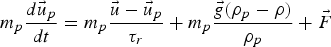


The spherical drag force proposed by Morsi et al. [21] is used in this study where particles are considered smooth and spherical. Stochastic tracking model (random walk) is used to include the turbulence dispersion of particles by integrating individual trajectories using instantaneous fluid velocity.
The explained approach (DPM) is used for both carbon particle and water droplet trajectory calculations. Furthermore, liquid droplets evaporation is modelled using a Convection/Diffusion Controlled sub-model [22] using the following expression when droplet temperature is lower than boiling point: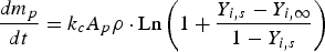


When the droplet temperature reaches the boiling point while containing mass that can evaporate, convective boiling of a discrete phase droplet is used for which the details and related equations can be found here [14].
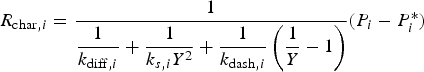
For carbon particle combustion, the Field Char Oxidation model is used which is a simplification of unreacted shrinking core modelling (USCM). The oxidant from the gas phase diffuses into the surface and reacts with solid core. The product layer (here ash) is produced on the surface and creates a product layer which increases the resistance of gas diffusion.
The combustion rate of solid carbon is modelled using DPM multiple surface reaction model and the rate is calculated from the expressions below [23]: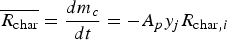


Here 


Geometry and grid
Computational grid for simulations and grid independency study.
More discussion on meshing and grid dependency is presented in Section ‘Model validation and grid independency’, but it is worth mentioning here that based on the results, medium size grid is used for the rest of calculations. A representation of computational grid for air quench section is shown in Figure 3. The advantage of using polyhedral cells is lesser cell counts compared to tetra and hexahedra elements while maintaining the accuracy of the predictions. The Equivalent tetrahedral cell type is also reported in Table 1 and as seen using polyhedral mesh can reduce the cell count by factor of 4.3 which cause a considerable reduction in computational costs. Air quench section for medium size grid, inner cross-section (left) and outer face (right).
Boundary conditions and model set up
Inlet boundary conditions (B.C)
Inlet boundary conditions for CFD model setup.
Another important consideration is species inlet profiles, which are not uniform. The oxygen is injected from sides in CCF and most of the remaining CO and H2 are concentrated in the middle of the flow at the outlet of CCF. The same non-uniform profiles can be expected for other species as shown in Figure 4. The profiles are obtained from another CFD model developed for CCF at Tata Steel, R&D. Species profile at the inlet of reflux chamber (average values are reported in Table 1).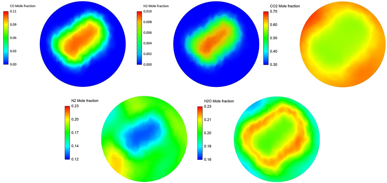
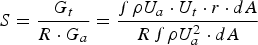
Also, the iron ore and oxygen injection into the CCF is not fully radial and injection ports are tilted with a tangential velocity component which causes a swirl motion. The swirl motion is convected upward to the reflux chamber. So the flow at the inlet of reflux chamber is not fully axial and has a swirl motion. The intensity of a swirl motion is characterized by swirl number (S) defined as the ratio of tangential momentum (


At the HIsarna pilot plant the water is sprayed through a two-fluid atomizer with nitrogen as carrier gas (blast atomizer). Little information was available regarding the atomizer specifications and geometry. The only available data were flowrates of nitrogen and water and the injection spray angle. So for water droplet injection, the data are set based on Poozesh et al. [24] which have studied experimental and numerical droplet size and velocity distribution of a two-fluid atomizer. The water droplet diameter is modelled using cone injection with a diameter of 9 × 10⁻⁵ m, injection velocity of 25 m s−1 and spray angle of 30 degree.
Wall boundary conditions and heat loss
The off-gas system walls are made of steel pipes (OD: 0.038 m, thickness: 0.005 m) through which counter-current cooling water flows to cool the wall. Due to a higher temperature inside the reflux chamber (compared to the rest of the off-gas system), and to protect the cooling pipes from thermal melting and stresses, a layer of refractory material on top of the cooling pipes is applied. Rows of anchors are placed on the circumference of pipes (same material as pipes) to firmly hold the refractory layer applied on top (Figure 5(A)). Wall layers for shell conduction model.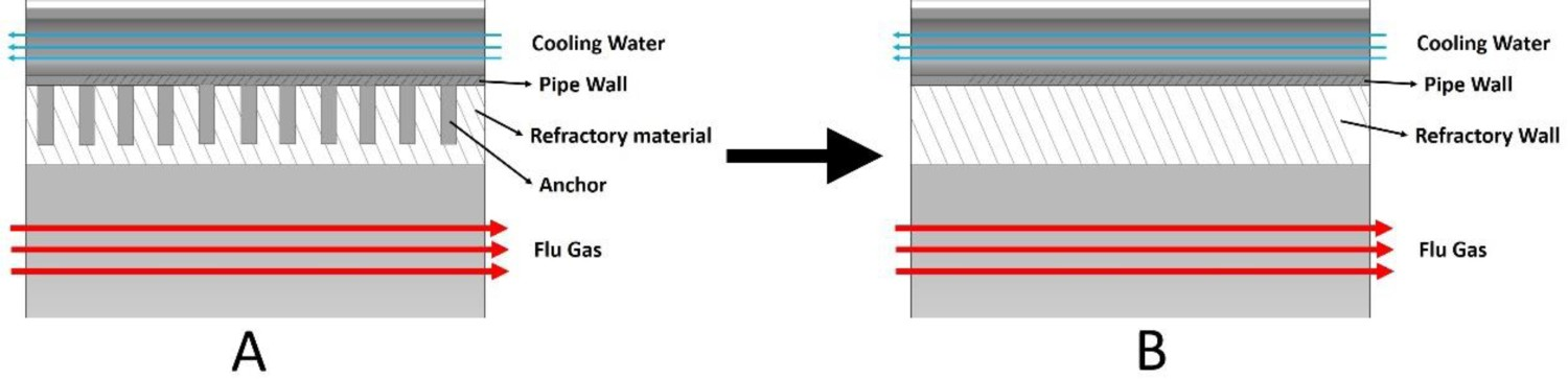
Incorporating details of the anchors and to directly resolve different layers of the reflux chamber wall in the CFD model will need a very fine computational grid which heavily increases the computational cost. To avoid that, the wall is modelled using shell conduction approach where different layers of the wall can be considered as a uniform layer in series with an assigned material and defined thermal and physical properties. This way, appropriate thermal resistance across the wall thickness is imposed and wall conduction is taken into account without considering the details of different wall layers in the geometry and computational domain. Above the reflux chamber only one layer representing the cooling pipe thickness with properties of steel is assigned for the wall. For the reflux chamber, an extra layer to represent the refractory wall is considered however, the material property assignment is not as straightforward as steel pipes.
The refractory wall can be considered as a composite of raw refractory material (matrix) and anchors (filler). This combination changes the thermal conductivity, density and heat capacity of the refractory wall with respect to the raw refractory material.
Wall material properties.
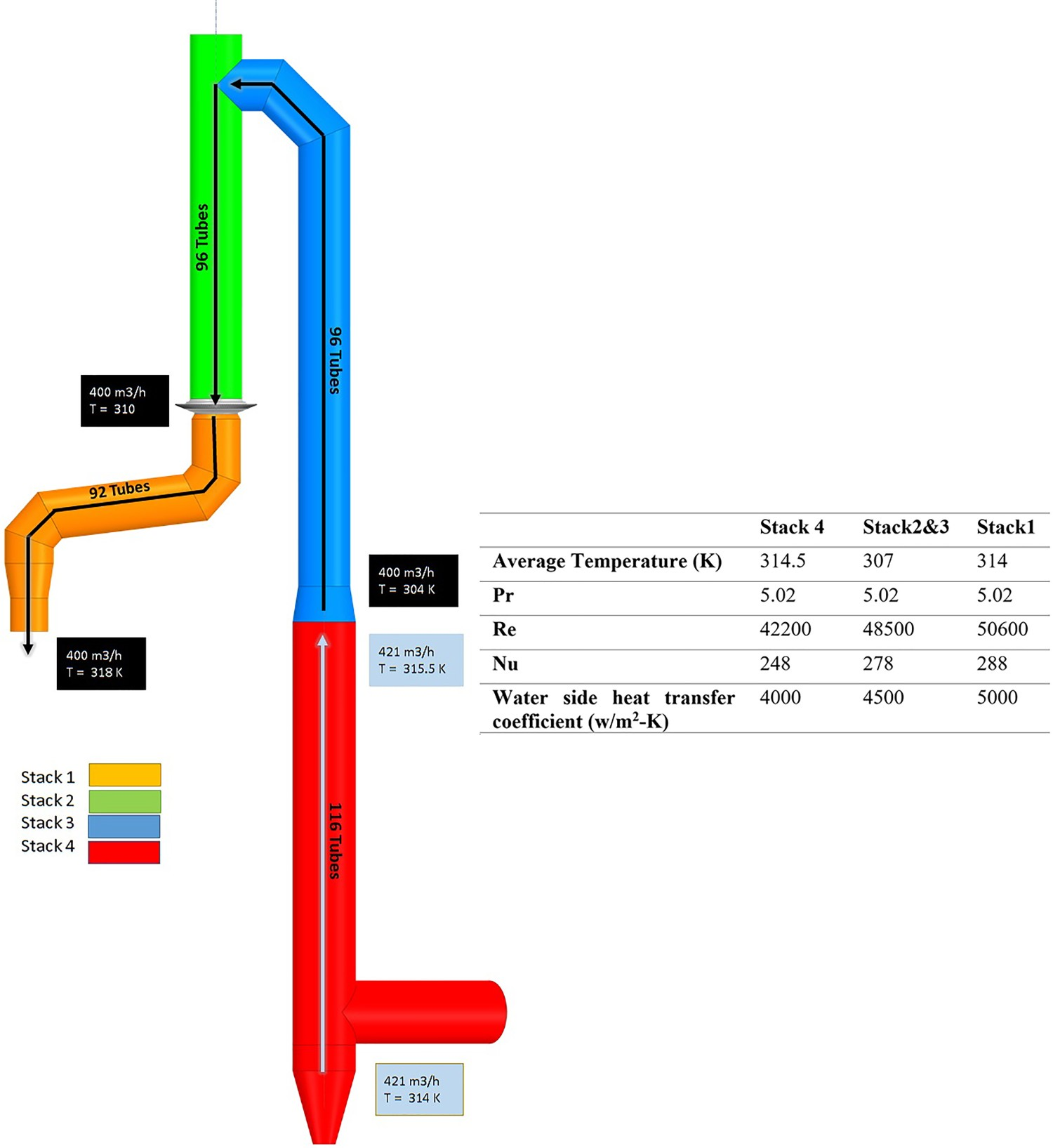
The cooling system is divided into four different cooling stacks. The cooling water flowrate and average temperature are shown in Figure 6. The heat transfer coefficient for the cooling water side is calculated for each cooling stack according to the Pak and Cho relation [25]: Off-gas cooling water circuit.
Reactions and kinetics
A detailed kinetic mechanism proposed by Cuoci et al. [13] is used for the CO–H2 mixture combustion. The mechanism contains 14 species and 33 reactions and it is validated using experimental data.
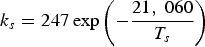
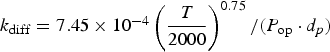
Three different reactions are considered for carbon combustion. The kinetic expressions are taken from the study of Wen et al. [23] in the form of Equation (21). The reactions and kinetic data are as follows:
where 


Model summary and solution procedure
Summary of models used in the study.
Numerical discretization of conservation equations is performed using the second-order upwind scheme. Ultimately a convergence criterion of 10−4 for the relative error between two successive iterations is specified.
Result and discussion
Model validation and grid independency
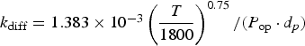
Figures 7 and 8 show the predicted temperature and compositions profile and comparison with industrial data. The data are plotted as an average value over a cross-section swept along centreline of the system (length). As seen, the predictions are in fair agreement with the measured industrial data (Figure 9). Temperature profile for model prediction and plant measurements (10% error in plant data). Composition profile for model prediction and plant measurements (dry basis). Composition at different measurement point.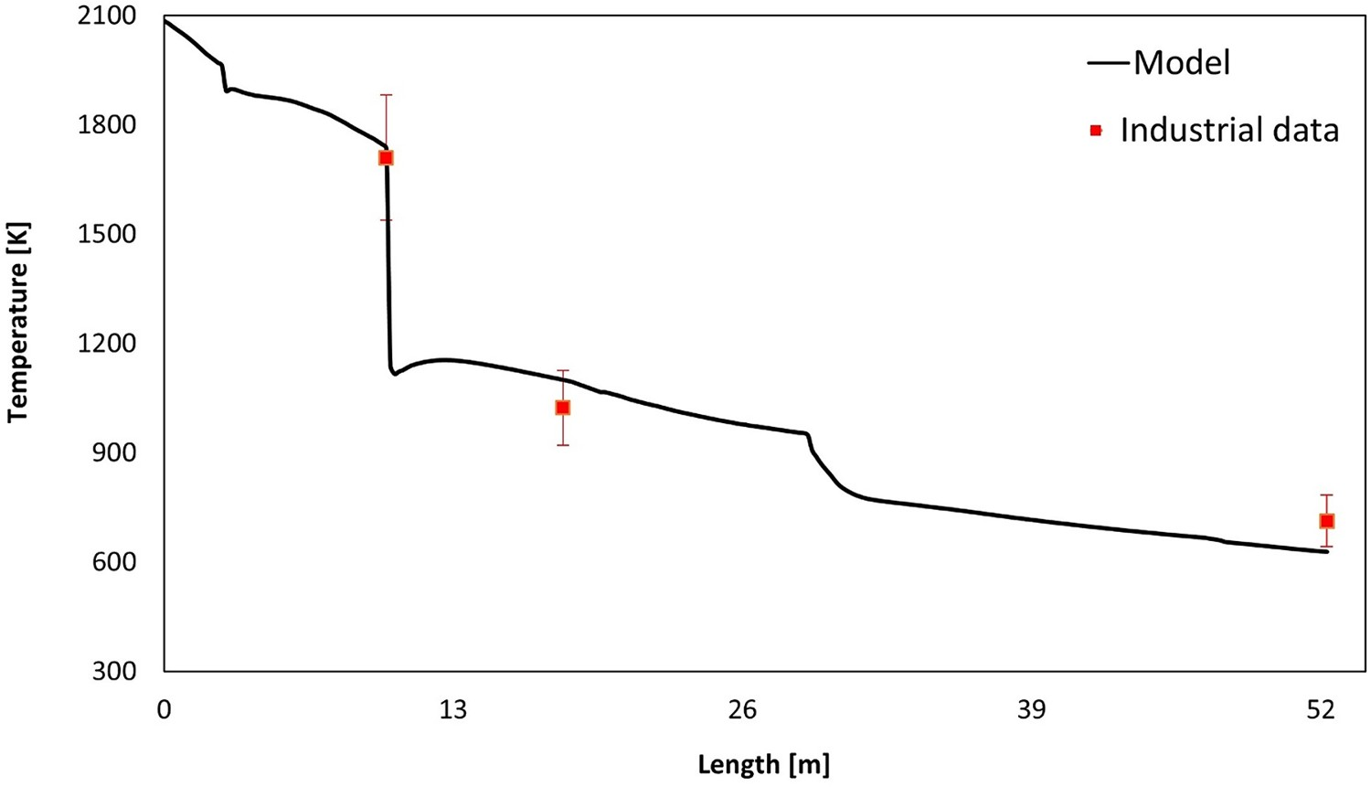
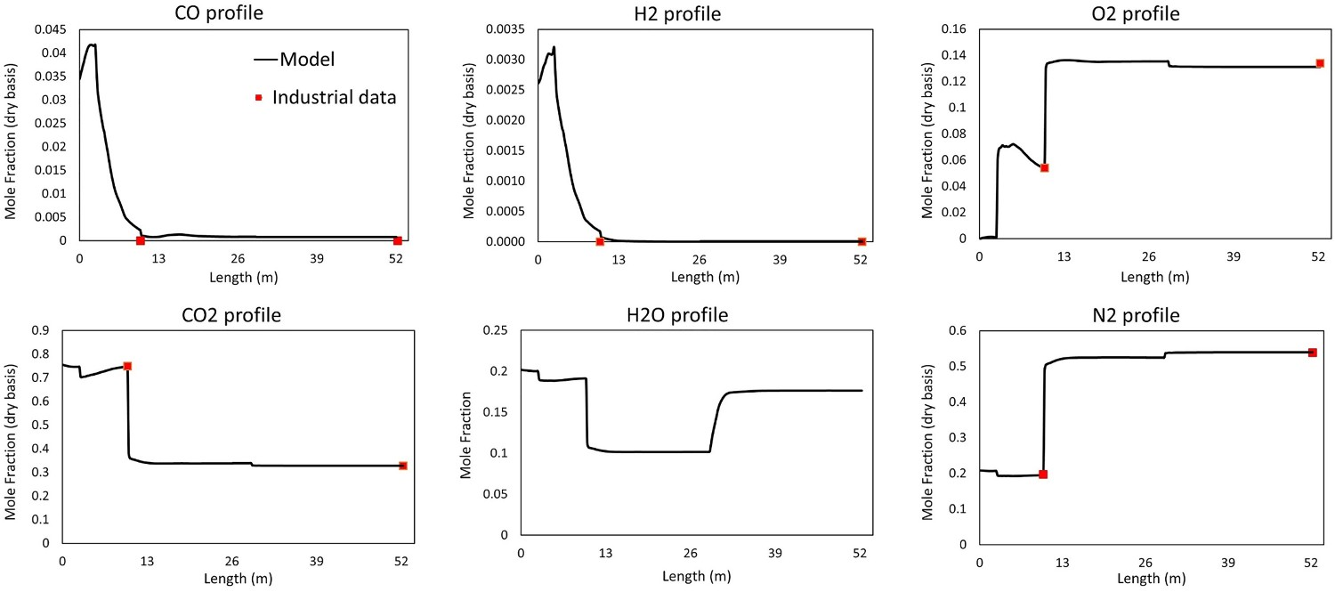
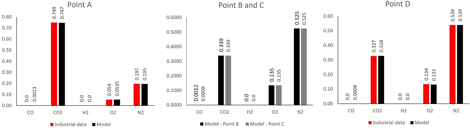
The composition values at different measurement points are also shown in Figure 10, these data are not available at points B and C. Composition and temperature contours at different cross-section over the off-gas length.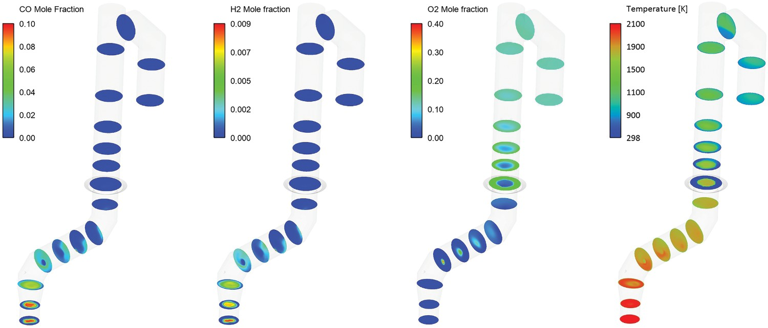
The grid dependency for different meshes was performed up to the water quench zone (point C) and there were few differences in final results between different computational grids presented in Table 1. The predicted profiles were quite similar in trend (not shown here for brevity), however, the coarse grid led to slightly higher temperature along the reflux chamber and up/down leg. For example, the outlet temperature of the reflux chamber (point A) and the temperature before the water injection (point C) for the coarse mesh were 30°C and 15°C higher than the other two grids, respectively. This difference was negligible for the medium and fine mesh.
To have a better analysis, contours of compositions and temperature are shown in Figure 10.
As evident from profiles and contours, the amount of CO and H2 is increasing before hitting the oxygen injection area (length: 3 m). This is mainly due to carbon reaction with H2O–CO2 mixture and also CO2/H2O thermal dissociation into CO and H2. Over the same length the temperature constantly decreases at a constant pace mainly due to heat losses through the wall, endothermic dissociation of CO2 and H2O and endothermic reaction of carbon with H2O–CO2 mixture.
Then there is a sharp increase in oxygen concentration where oxygen is injected (length 3 m) in the reflux chamber with a drop in temperature. CO and H2 are burned with a sudden drop in mole fraction profile. Oxygen is reduced as its consumed for the combustion and the amount of CO2 and H2O is increased as product of the combustion. Temperature is constant at first after the oxygen injection point due to the heat from combustion but again reduces due to heat losses through the wall and other endothermic reactions. There will be another sharp increase in oxygen profile and drop in temperature which is related to the air injection through air quench channels (length 10 m).
Downstream, where flue gas is quenched with water (length 29 m), there will be another steep reduction in temperature due to evaporative cooling. More discussion on water quenching is presented in Section ‘Effect of water injection’.
Another important point is the effect of air quenching. As mentioned before, beside quenching the flow, one more benefit of quenching with air is freezing the molten particles escaping from CCF and reflux chamber. As seen from the temperature contour, the injected air creates a cool ring near the wall and once the particles reach this cold zone, they freeze. The frozen particles are carried away with the flow and will not accrete on the wall.
This can also be seen from Figure 11 where flow streamlines coloured by temperature are shown. The swirl motion of the flow at the inlet can also be confirmed from the streamlines (S = 0.6). Flow streamlines coloured by temperature – effect of swirl motion.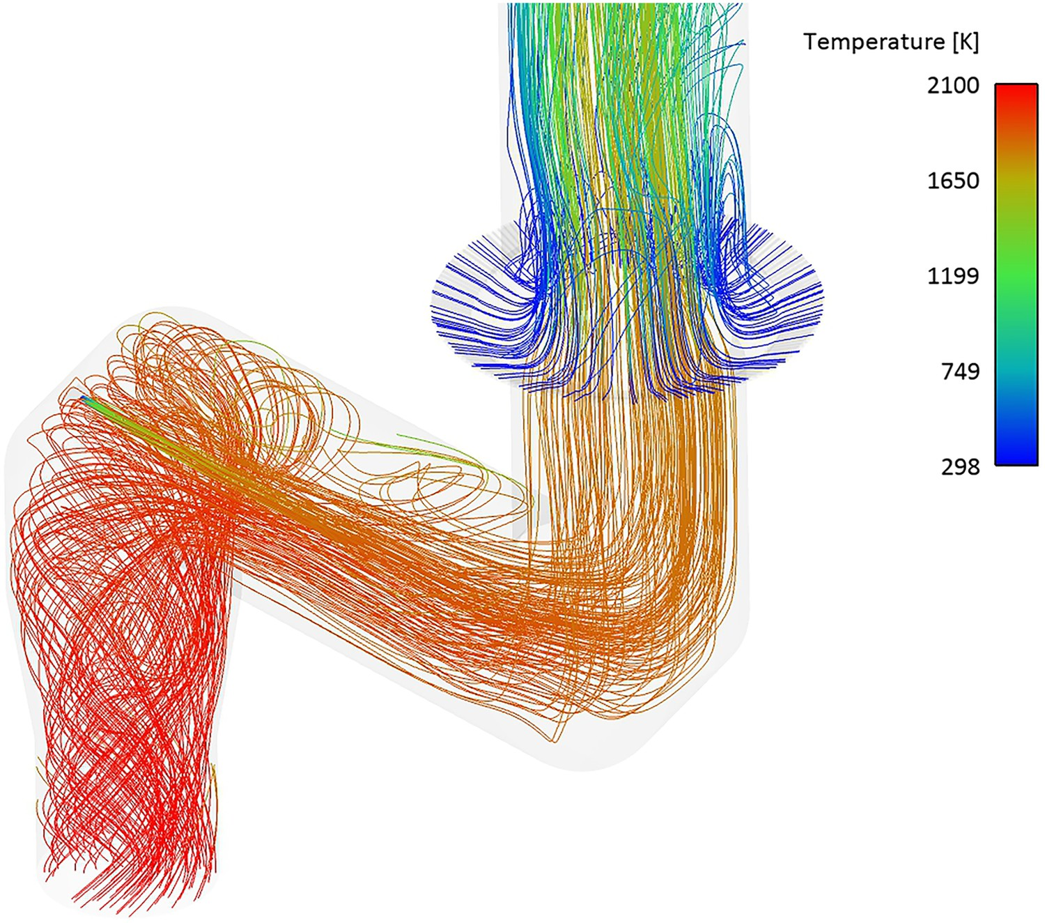
Calculated heat losses are reported in Table 5 and compared with available measurements. The total heat loss is predicted to be higher. One reason is that at the pilot plant only the heat loss to the cooling water is measured and other losses (pipes and connections) are not measured, so practically the real heat loss in the plant will be higher than the measured heat loss. On the other hand, the model considers 100% of the loss to the cooling water which is the main reason for this difference. The heat removed from the flue gas by evaporative cooling is around 1.2 MW which is a considerable.
The contours of wall temperatures are shown in Figures 12 and 13 for the reflux chamber and air quench respectively. The inner wall refers to a wall layer in contact with flue gas and outer wall in contact with cooling water. The average values of the wall temperatures are reported in Table 6. There is a notable temperature difference between inner and outer wall of the reflux chamber (1070°C difference) which shows good isolation properties of the refractory. This is necessary since the temperature is high in the reflux chamber which would cause the cooling pipes to melt without refractory. Above the reflux chamber, however, there is a slight difference between the inner and outer wall temperature as the flow is quenched and only steel tubes are used as cooling wall with a very thin thickness of 5 mm. Reflux chamber inner (left) and outer (right) wall temperature distribution. Air quench inner (left) and outer (right) wall temperature. Heat loss prediction versus industrial data. Average wall temperature – model prediction.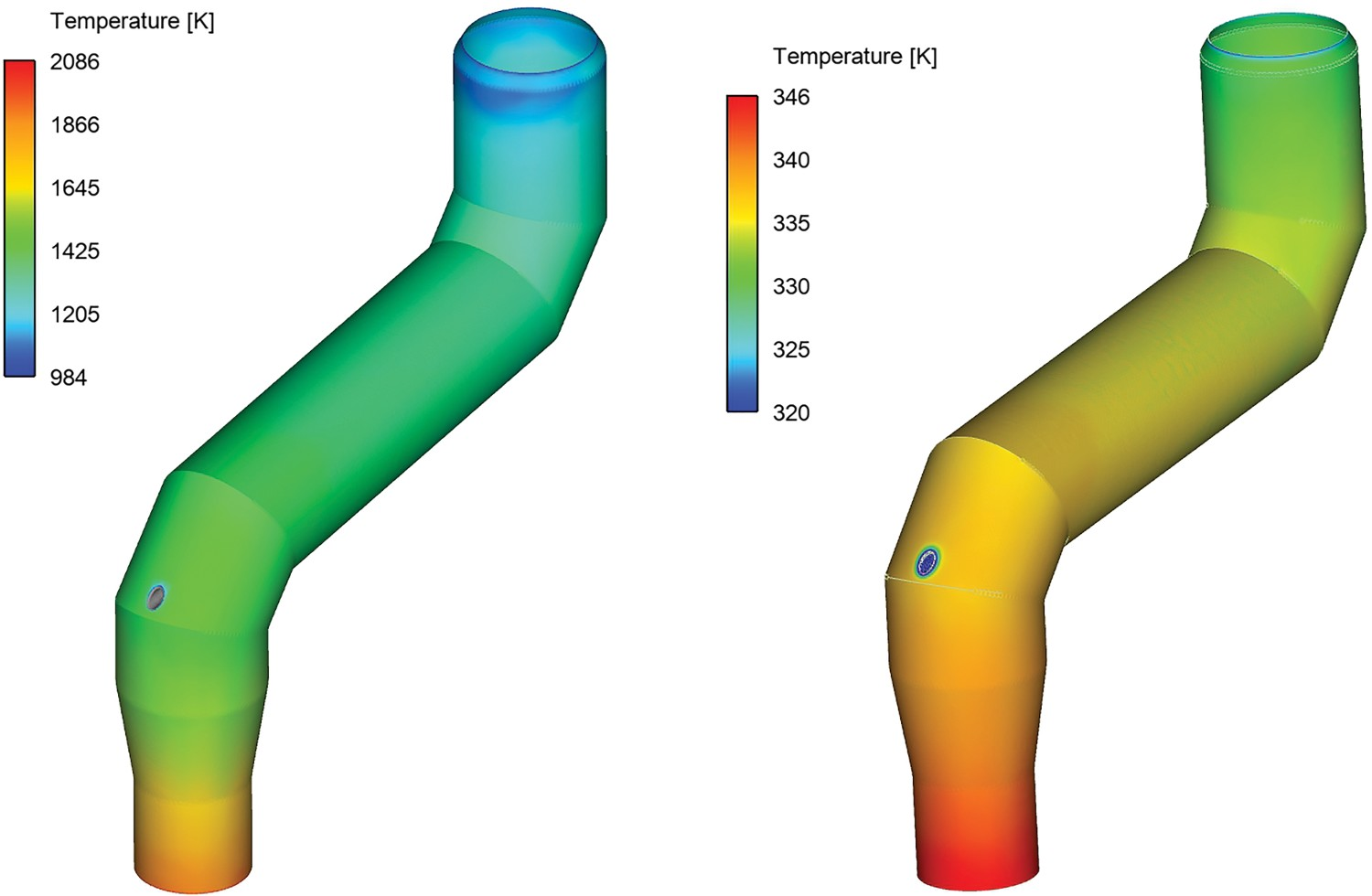
Effect of carbon particle reaction
Figure 14 shows the carbon particle tracks scaled and coloured by particle diameter. As shown, the particles are gradually depleted of carbon and reach minimum diameter. The maximum carbon conversion ( carbon particle track and predicted conversion at measurement points (refer to Figure 2 for measurement points precise location in the off-gas).
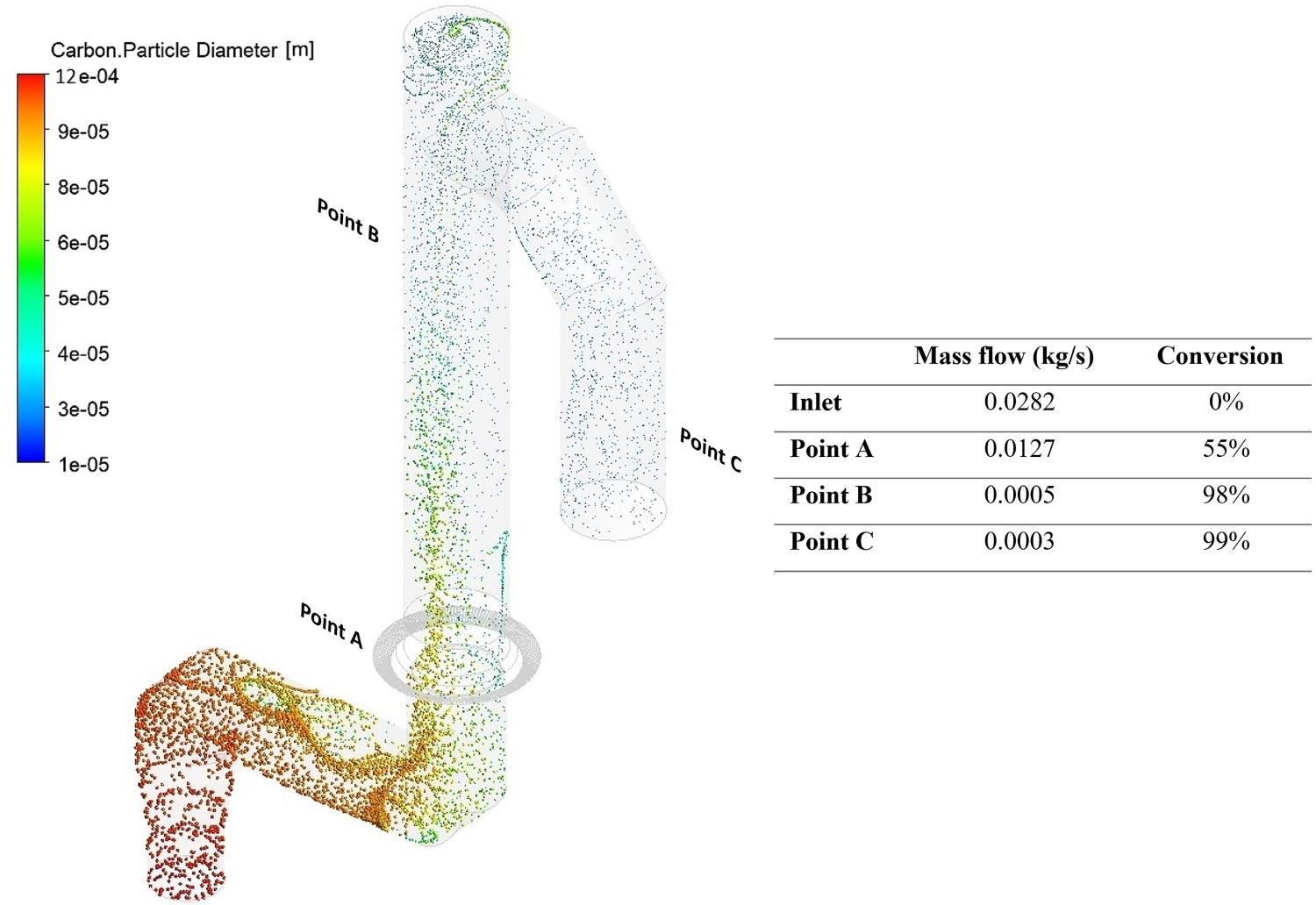
The conversion of carbon is highest inside the reflux chamber, considering the shorter length compared to up leg and down leg. This is due to pure oxygen injection inside the reflux chamber at relatively higher gas temperature which causes the gas–solid reactions to proceed at a higher rate. The air quench also plays an important role in combusting carbon particles and CO–H2 mixture, and basically any left over from the reflux chamber is safely burned in the up leg and down leg section. Ultimately all carbon is consumed before reaching the water quench zone (Point C).
Incorporating carbon combustion reactions in the model will change the temperature and composition profile compared to a case without considering any gas–solid reaction. To explain the importance of this consideration, a simulation is performed where only gaseous reactions are considered, neglecting carbon particles flow and reactions in the model. The temperature and composition profiles are shown in Figure 15 and as is shown it shifts up by considering carbon particle reaction as the overall gas–solid reaction is highly exothermic. The temperatures at points A, B and D are around 60°C higher when gas–solid reactions are considered. The effect is also notable in CO and H2 profile which are higher by considering carbon particles as they participate in H2–CO generation. It also has a considerable effect on O2 profile. When carbon particles are not considered the profile in the reflux chamber is constant as the consumption of oxygen halts when the CO–H2 mixture is fully combusted. When carbon particles are considered, the oxygen inside the chamber is reduced along the length as it is constantly consumed by produced CO–H2 from carbon reaction with O2, H2O and CO2. In conclusion, considering carbon particles in the model has a notable effect on temperature and composition profiles and leads to a better fit with industrial measurements. However, incorporating gas–solid reactions using DPM model can significantly increase the calculation time. Effect of gas–solid (carbon) reaction on averaged cross-section composition and temperature profiles (modelled up to Point C).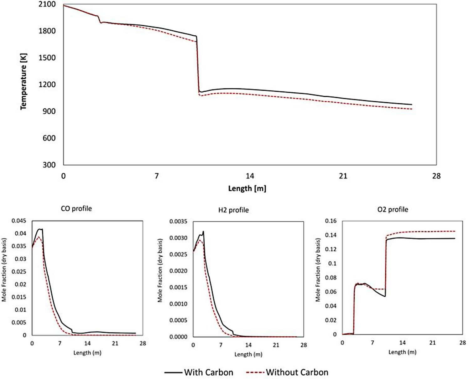
Effect of water injection
Figure 16 shows a graphical representation of how the water spray is modelled inside the off-gas system. The gradual decrease of particle diameter due to evaporation is also very well shown. Water injection through cone spray model – droplet tracks in down leg.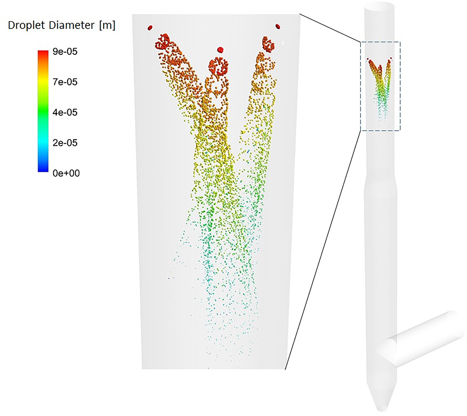
As reported in Table 4, the amount of heat removed by evaporative cooling is considerable (1.2 MW). The water injection can make a temperature difference of 120°C compared to a case without water injection (quenched only with nitrogen) as shown in the temperature profile of Figure 17. Effect of water injection on composition and temperature profiles in down leg.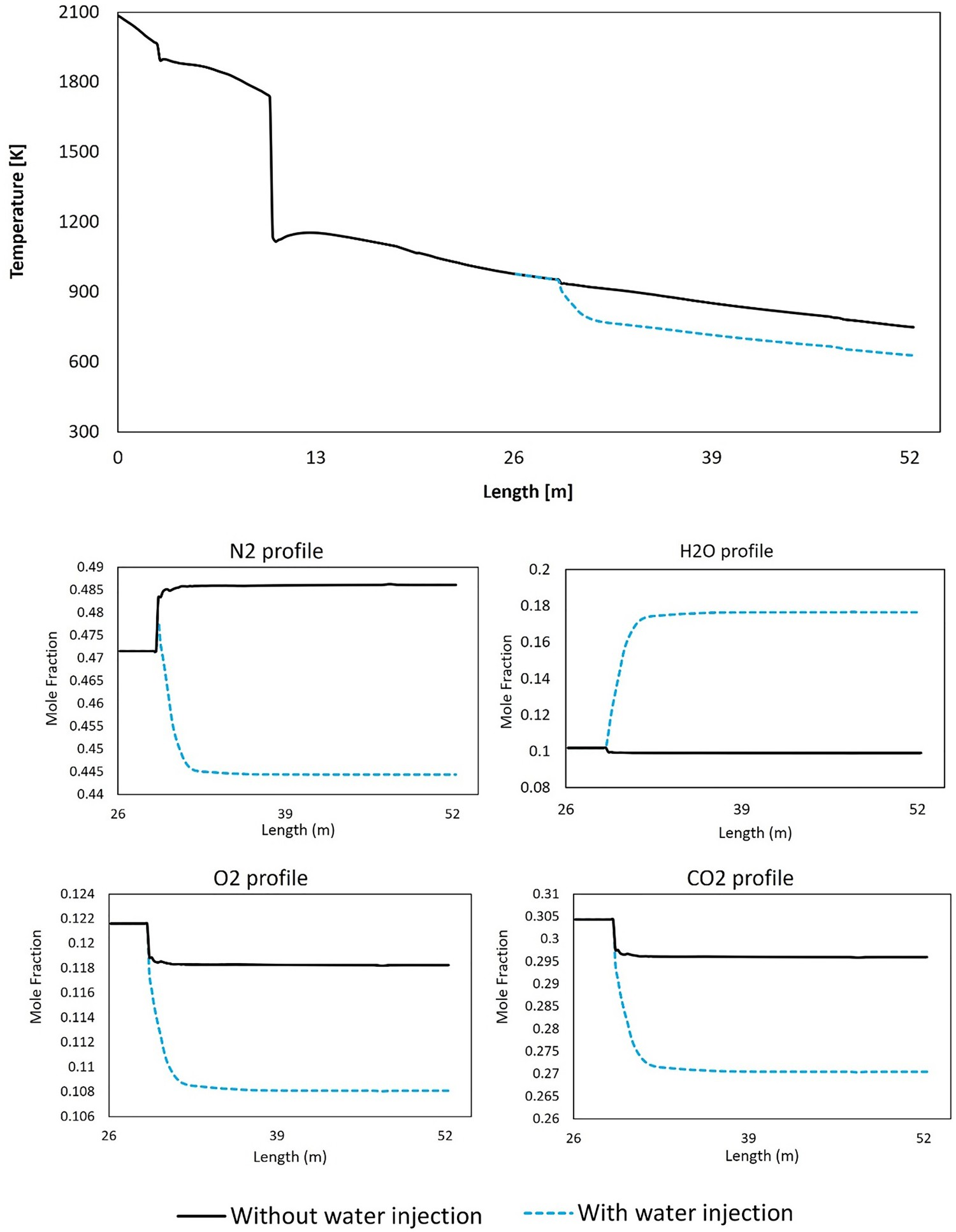
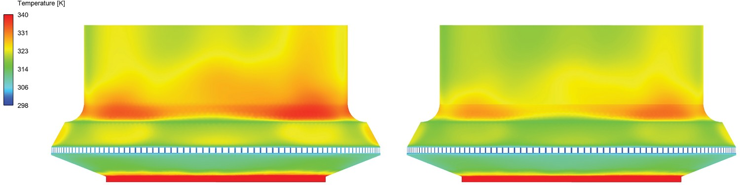
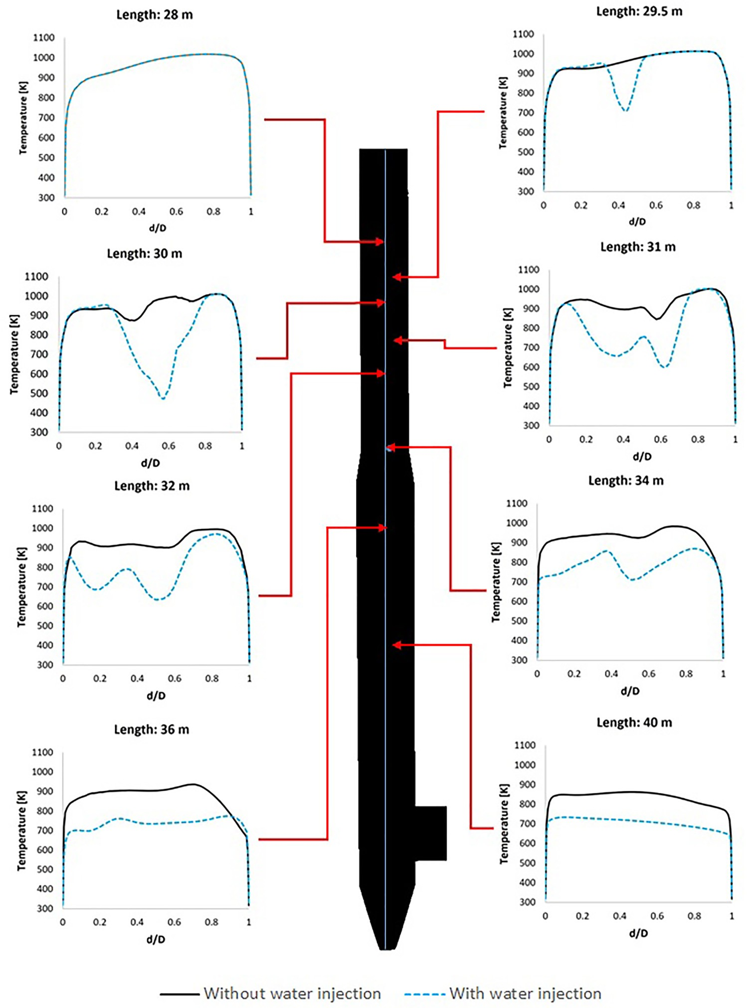
For a better graphical representation, the effect of water quenching on temperature and water vapour contours are also shown in Figures 18 and 19 which show cross-sectional temperature profiles over the pipe diameter ratio (d/D). Since the spray angle is not wide and also due to the high flowrate of the flue gas, the water droplets are not well-spread at the beginning of the injection and cold spots with a much lower temperature than the surrounding are formed. This can be seen from Figure 19 where the temperature drops fast and takes a V-shaped profile with low local temperature at the centre. This phenomenon is better shown in temperature contours of Figure 18. The temperature contour at each cross-section reaches a constant shape with uniform profile downstream as water is fully evaporated. Composition and temperature contours at different cross-section in down leg – effect of water injection. Temperature profile at central line on different cross-section and at different length.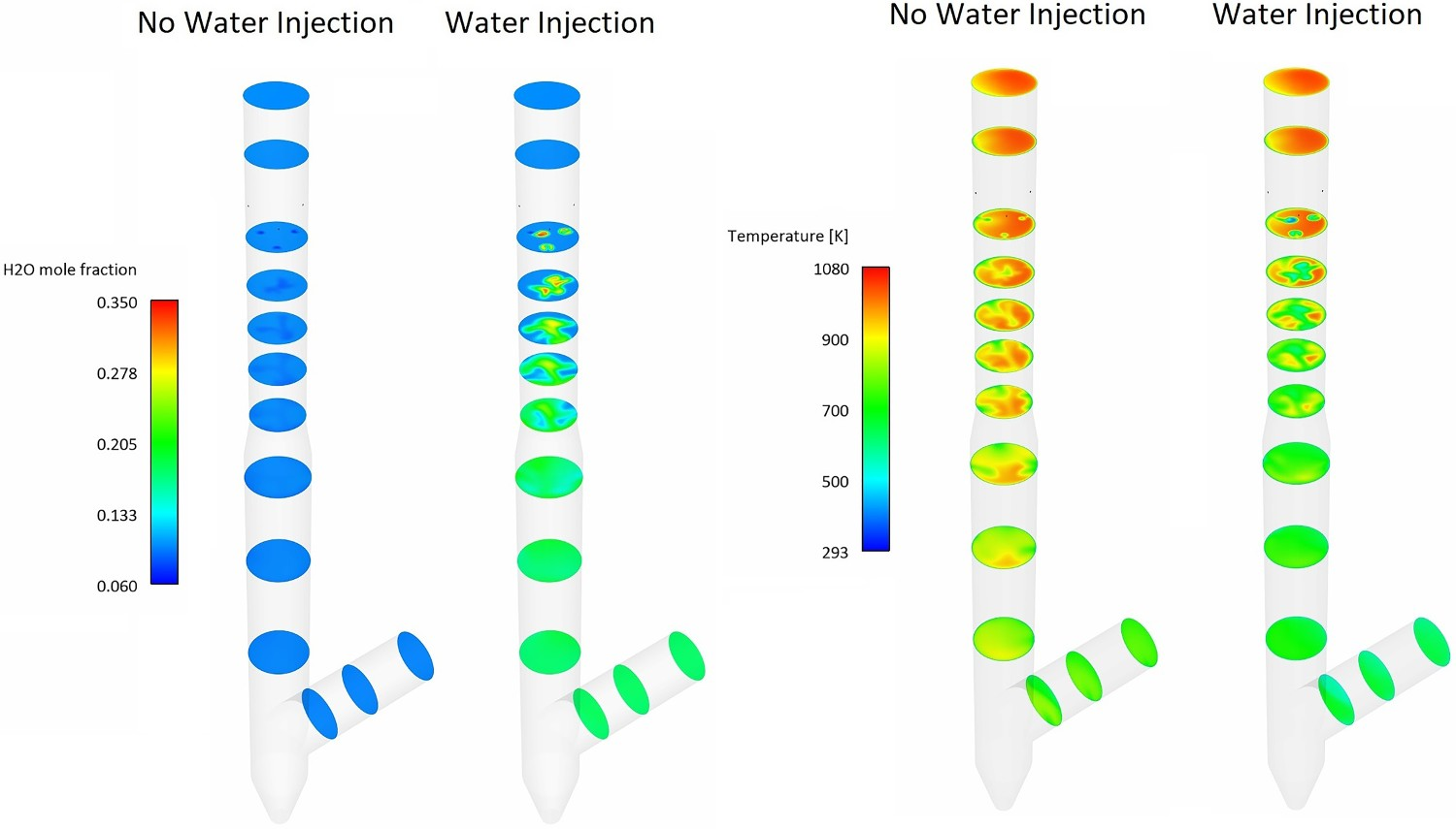
The wall temperature will also decrease locally by water injection as shown in Figure 20, however, the average wall temperature change is not noticeable. Down leg inner wall temperature distribution – effect of water injection.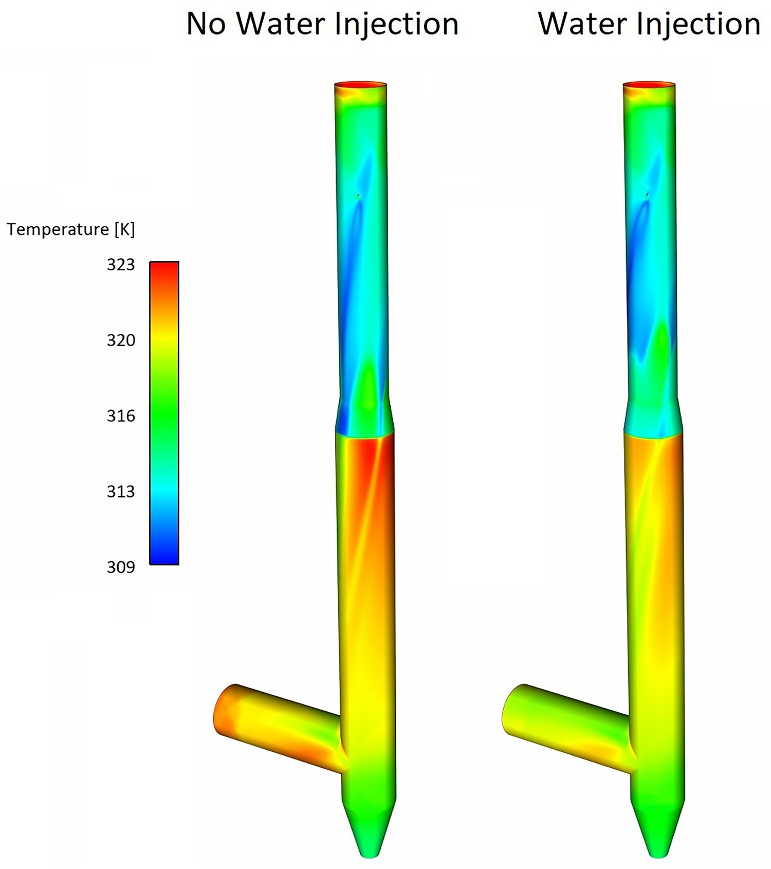
Effect of oxygen injection
From the oxygen composition profile (Figure 8), a sharp increase in oxygen mole fraction is observed in the reflux chamber (outlet 5.4% oxygen).
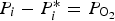
With a simple theoretical calculation for overall reactions of 


Due to the limited length of the reflux chamber, achieving full combustion of unwanted elements is not possible at the current plant installation and the combustion is only partial in the reflux chamber (55% and 95% conversion for carbon and CO–H2 respectively predicted by the model). The rest is combusted in the up leg as the temperature is still high enough and oxygen is available in a large amount by injecting air through the air quench. So leakage of CO and carbon from reflux chamber seems to be fine as long as the escaped fractions are combusted downstream. On the other hand the oxygen is injected in pure form (99.5% purity) into the reflux chamber which, unlike air quench, that uses ambient air, involves certain costs. So it is desired to reduce pure oxygen injection to reduce operating costs as much as possible.
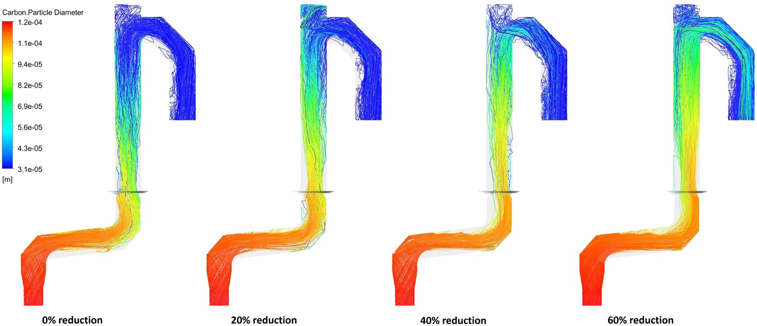
A set of simulation is performed to see the effect of oxygen injection reduction (20%, 40% and 60% reduction) on mixture conversion. Figure 21 shows the CO and O2 mole fraction at different measuring points along with CO and carbon conversion. As shown, reducing oxygen injection will increase CO mole fraction, reduce O2 mole fraction and consequently reduces the CO and carbon conversion at the reflux chamber outlet (point A). Up to 40% reduction in oxygen, carbon is still fully combusted before reaching point C as shown in Figure 22 illustrating particle tracks coloured by particle diameter. However, carbon escapes when oxygen injection is reduced by 60% and enters the water quench zone (97% conversion). CO mole fraction at point C is increased (lower conversion) by reducing oxygen injection into the reflux chamber. It is risky to let a high amount of CO enter the water quench zone where combustion is more likely to halt as the temperature drops fast and below the auto-ignition point of CO (882 K) CO–O2 mole fraction and carbon conversion for different oxygen reduction cases. Carbon particle track, coloured by particle diameter for different oxygen reduction cases.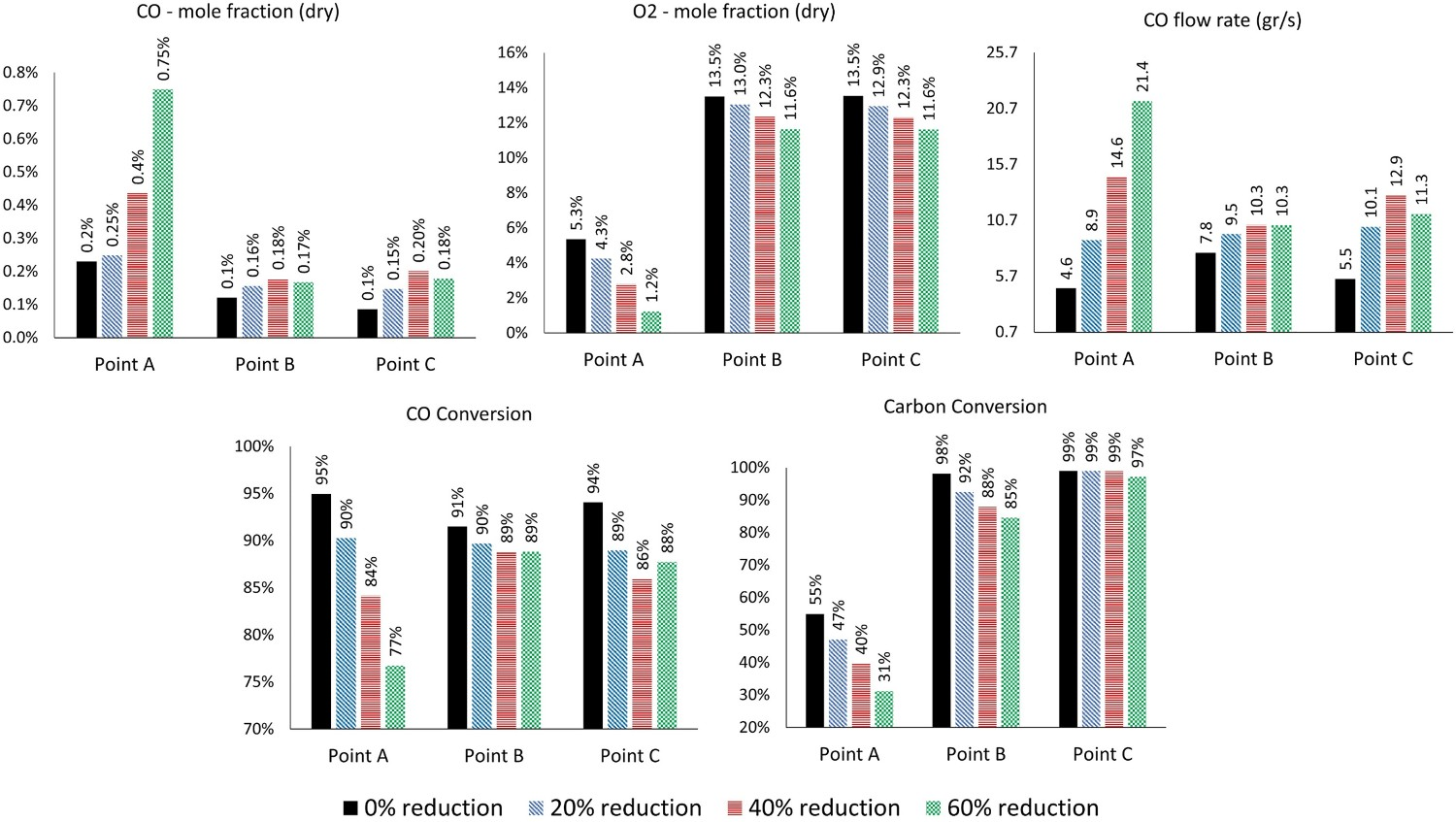
To have a better understanding, a quick analysis using CHEMKIN software where a mixture, containing a certain amount of CO (same as point B), with the same combustion mechanism as used in the CFD models, is performed to investigate the auto-ignition properties using closed homogeneous reactor model. The initial temperature of the mixture is fixed, and temperature increase and CO consumption are monitored. The results are shown in Figure 23 and one can conclude that the ignition (increase in temperature and initiation of CO consumption) is delayed by reducing the temperature and there is no ignition below temperature of 882 (609°C). At 882 K, even though the ignition starts, the consumption rate of CO and temperature increase rate are quite low, and for the time analyzed (30 s) full consumption of CO could not be achieved. To make sure that all CO is combusted, a higher temperature than the auto-ignition temperature (around 200°C higher) is desired. Temperature and CO mole fraction transient profile for auto-ignition analysis.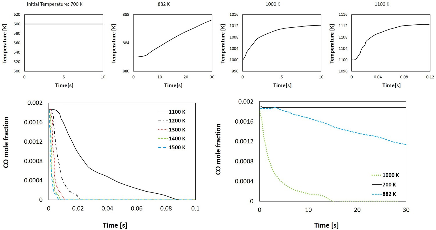
So reducing oxygen injection is possible, but it should be in a quantity that the unwanted species (CO and carbon) are still combusted at a higher temperature than the auto-ignition point and avoiding a large amount of CO into the off-gas sections where the temperature is lower. From model predictions any reduction in oxygen injection will increase the CO flow rate (and mole fraction) entering the cold region of the off-gas. In conclusion the amount of reduced oxygen depends on the environmental regulations and the amount of permitted CO emission.
Conclusion
A 3D CFD simulation of the HIsarna off-gas system is performed. The effects of different operating parameters are investigated and the following conclusions are drawn: The developed CFD model is capable of providing detailed information on the flow behaviour, conversion of unwanted species, and heat transfer within the reflux chamber and is in good agreement with available plant data. Incorporating carbon particle and related gas–solid reactions change the thermal and composition profiles along the system length. It increases the average temperature at measurement points and increases the oxygen consumption inside the reflux chamber. The water injection has a notable effect on composition and temperature profile in the down leg. The temperature reduction is predicted around 100°C once water is injected which makes the flue gas condition proper for further cooling and ultimate treatment in the sulphur removal unit. The oxygen is injected with 120% excess to ensure complete conversion of unwanted species. Even with this excess, from both plant data and model results, complete conversion of CO and carbon cannot be achieved in the reflux chamber. The escaped CO and C from the reflux chamber are converted in the up/down leg as the temperature and oxygen concentration is still high to proceed the combustion reaction. However, from model predictions, it was observed that oxygen injection can be reduced while achieving full conversion downstream. Too much reduction in oxygen injection will cause CO and carbon to enter the water quench zone where the temperature falls under the auto-ignition of CO and will lead to unwanted pollutant emission.