Social Media's Impact on the Consumer Mindset: When to Use Which Sentiment Extraction Tool?

Abstract

User-generated content provides many opportunities for managers and researchers, but insights are hindered by a lack of consensus on how to extract brand-relevant valence and volume. Marketing studies use different sentiment extraction tools (SETs) based on social media volume, top-down language dictionaries and bottom-up machine learning approaches. This paper compares the explanatory and forecasting power of these methods over several years for daily customer mindset metrics obtained from survey data. For 48 brands in diverse industries, vector autoregressive models show that volume metrics explain the most for brand awareness and purchase intent, while bottom-up SETs excel at explaining brand impression, satisfaction and recommendation. Systematic differences yield contingent advice: the most nuanced version of bottom-up SETs (SVM with Neutral) performs best for the search goods for all consumer mind-set metrics but Purchase Intent for which Volume metrics work best. For experienced goods, Volume outperforms SVM with neutral. As processing time and costs increase when moving from volume to top-down to bottom-up sentiment extraction tools, these conditional findings can help managers decide when more detailed analytics are worth the investment.

“In a world where consumer texts grow more numerous each day, automated text analysis, if done correctly, can yield valuable insights about consumer attitudes”

Humphreys and Wang (2017)

From banks to potato chips, from large (e.g., J.P. Morgan) to small (e.g., Kettle) brands, the growth in the amount of available online user-generated content (UCG) provides managers with rich data opportunities to gauge (prospective) customers’ feelings. The Markets and Markets (2017) report shows that more than 75% of companies employ social media analytics by collecting and using the volume and valence of UGC to monitor brand health. To do so, most companies either purchase processed social media data from external providers (e.g., Social Bakers) or use off-the-shelf software solutions such as Linguistic Inquiry and Word Count; (LIWC). To date, most academic studies either solely rely on volume metrics (or pre-SET metrics) ¹ (Srinivasan, Rutz, & Pauwels, 2015) or choose a single sentiment extraction tool (SET), such as dictionary-based analysis (Kupfer, Pähler vor der Holte, Kübler, & Hennig-Thurau, 2018; Rooderkerk & Pauwels, 2016) or machine learning-based techniques (Büschken & Allenby, 2016; Homburg, Ehm, & Artz, 2015). As pointed out by Balducci and Marinova (2018), few studies have provided a detailed explanation for their choice of a specific SET. The absence of a comparison is unfortunate for researchers and marketing practitioners because it hinders the ability to draw empirical generalizations and develop a consistent body of knowledge.

1

We thank the anonymous reviewer for this term

Does the choice of SET matter? Yes, for two reasons: UCG is often ambiguous and SETs substantially differ in their underlying approach to classifying sentiments in positive, negative or neutral categories. Pre-SETs only track classic volume-based metrics, such as the number of likes, comments or shares – with the assumption that more of such “engagement” is better for the brand. Top-down approaches as described by Humphreys and Wang (2017) use linguistic dictionary-based software solutions, such as LIWC, which rely on word lists that count the number of pre-classified words that belong to different categories (positive or negative emotions). Bottom-up approaches rely on machine learning and artificial intelligence in combination with training data to infer the probability that certain words or word combinations indicate a positive or negative sentiment.

Examples abound on ambiguous UGC, such as “@Delta Losing my bag is a great way to keep me as a customer,” which got much “engagement.” Human coders correctly deduce that the post conveys negative sentiment. However, a volume-based pre-SETs would reflect a simple count of, e.g. likes, comments and shares, and a simple top-down dictionary-based SETs would classify it as positive sentiment, given the higher frequency of positive words (great, keep me as a customer) over negative words (losing). In contrast, a bottom-up approach could classify the post as negative, but would require content-specific training data (i.e., “losing my bag” is especially harmful in the airlines context) which can be difficult to obtain and update.

These approaches come with certain benefits and costs and present a varying level of complexity for managers. Classic volume-based pre-SET metrics such as likes, comments and shares are easy to collect, relatively easy to implement into existing dashboards and fast to process. For example, once a manager has access to their brand Facebook account, the time and effort to collect such metrics is minimal. Thus, we posit that pre-SET volume metrics have low level of complexity. Still, their ability to capture all facets of human speech must be considered to be limited as outlined by our above example. Top-down approaches typically rely on “pre-manufactured,” non-contextualized word lists, provided by different commercial sources. Such top-down approaches require a medium level of effort in data preparation and computational power. Thus, they have medium level of complexity. However, given the lack of contextualization, they may lead to misinterpret the content as outlined in our example. In contrast, bottom-up approaches efficiently overcome the problem of contextualization. By using case specific training data, machine learning can infer specific word-combinations, which may be unique to a given context. This ability however comes at high costs as training data needs to be carefully collected, maintained and updated. While in some cases, managers could have access to “pre-manufactured” approaches which can be applied in their context, most of the time such on-the-shelf solution might not be available. Some discussion of this is warranted In addition, developing a meaningful machine-learning approach requires substantially more time and computational effort. Accordingly, such approach has a high level of complexity.

Hence, the dilemma: which SET should be used in these different situations?

The marketing literature does not yet provide managers with guidance on which SETs best predict key brand metrics, such as awareness, consideration, purchase intent, satisfaction and recommendation – the traditional survey metrics they are sometimes claimed to replace (Moorman & Day, 2016, p. 18; Pauwels & Ewijk, 2013). Studying the antecedents of these brand metrics is important as they are important predictors of sales and firm value (Colicev, Malshe, Pauwels, & O'Connor, 2018; Srinivasan, Vanhuele, & Pauwels, 2010). For example, while Colicev et al. (2018) extensively studies the effects of social media volume and valence on consumer and stock market metrics, they exclusively rely on a bottom-up Naïve–Bayes classifier to extract sentiment from social media posts. The research gap is especially harmful because marketers give increasing weight to UGC and its derived sentiment metrics in dashboards and decision making (Markets & Markets, 2017). UGC and its text analysis can yield valuable insights about consumer attitudes (Moorman & Day, 2016), but only if done correctly (Humphreys & Wang, 2017). What “done correctly” means could depend on the brand and industry. For example, sophisticated SETS may be more important to lesser-known brands than to well-known brands that professionally manage their social media presence. Likewise, search versus experience goods may experience different benefits from different SETs. Finally, industries with mostly negative UCG sentiment, such as airlines and banking, may only need volume-based metrics that serve as a cheap and fast proxy to explain consumer mindsets. In sum, managers and other decision makers (such as investors) are uncertain as to which SETs are more appropriate for a specific brand in a specific industry.

To address this research gap, we compare the most commonly used SETs in marketing in the extent to which they explain the dynamic variance in consumer mindset metrics across brands and industries. Our unique dataset combines, for several years, daily consumer metrics with Facebook page data for 48 brands in diverse industries, such as airlines, banking, cars, electronics, fashion, food, beverages and restaurants for a total of 27,956 brand-day observations. With an R-based crawler, we collected more than 5 million comments on brand posts for our brand sample and then extracted sentiments from this textual data. Using the most readily available measures of social media sentiment, we collected the pre-SET metrics of volume (number) of likes, comments and shares of brand posts. Next, we employed dictionary- and machine learning-based techniques to extract sentiment from the textual data (user comments and posts on brand Facebook pages). Using variables at the daily level, our econometric analysis addresses our research questions: (1) Which SET relates better to each consumer mindset metric in the consumer journey, specifically, brand awareness, impression, purchase intent, satisfaction and recommendation? and (2) How do brand and industry-level variables moderate these effects?

Research Background and Sentiment Extraction Techniques

Marketing scholars can use several tools to extract sentiments from textual data. Because some of these tools are not known to a broad audience of marketing researchers, we first discuss the range of available tools before focusing on the specific tools that are used in this study.

Different schools of research have aimed to identify and measure sentiments that are hidden in texts. Linguistics and computer science share a long history of analyzing data from textual sources, which is commonly referred to as Natural Language Processing (NLP). Independent from their scientific roots, the vast majority of sentiment and text analysis approaches rely on so called part of speech tagging, where the main text (often referred to as corpus) is divided into tokens, which are sub-parts of the main corpus. Tokens may be single words, complete sentences of even full paragraphs. The tokenized text is then fed into the text analysis tool that infers meaning from it. Part-of-speech tagging procedures assign tokens into categories, which could be word classes (e.g., subjects or verbs). Besides grammatical categories, tokens may also be assigned into pre-defined categories such as e.g. positive or negative emotions, anxiety or arousal. As text data are prone to noisiness and given that many common words do not provide meaningful information, the text data gets often cleaned by removing so-called “stopwords” that do not provide meaning (e.g., articles or numbers) and by reducing words to their stemmed form. To infer sentiment from tokenized text, two main approaches are available. Top-down approaches (e.g., LIWC) rely on dictionaries, which are lists that contain all words assigned to a specific category. By counting how many times a token (e.g., word or word combination) of a specific category occurs, the top-down approaches determine the strength of a specific content dimensions (e.g., positive sentiment).

In the case of bottom-up approaches, a-priori dictionaries do not exist and instead, a machine is trained to build its own list with the help of training data. Training data may origin from different sources. Whereas some studies rely on human coded data (Hartmann, Huppertz, Schamp, & Heitmann, 2019), where multiple coders classify a subsample of texts into categories, such as, e.g., positive or negative sentiment, other studies have used user generated content (see e.g., Pang, Lee, & Vaithyanathan, 2002), such as, e.g., online reviews where the additionally provided star rating provides the likely type of sentiment (i.e., 1 star indicates negative sentiments and 5 star ratings indicate positive sentiment). Then algorithms determine the likelihood that a document belongs to a specific category (e.g., positive emotion) based on the occurrence of a specific tokens from the tokenized text. To determine these likelihoods, the machine needs pre-coded training data (i.e., the human coded or review texts) with documents clearly belonging to each dimension (e.g. documents with only positive or negative sentiments). The machines then estimate the likelihoods of a text belonging to a category given the occurrence of specific tokens.

Top-Down Approaches

Top-down approaches are based on frequencies of occurrence of specific tokens (e.g., words) in text. Basic “grammatical” word categories originate from speech tagging, which assigns words into 9 main categories (e.g., nouns, verbs, articles etc.). Words can also be assigned to other dimensions such as sentiment (e.g., LIWC positive and negative sentiment) or more specific dimensions such as fear, anger, anticipation or joy. To do so, for instance, Mohammad and Turney (2013) use NRC dictionary approach included in the EmoLex software, while Ribeiro et al. (2016) compare 24 popular commercial software choices of such sentiment analysis.

Researchers may use existing word lists or tailor the lists for the research context, industry or product category. Such tailoring requires a high level of expertise, availability of skilled coders as well as enough material to infer all words that are related with the construct (e.g., Mohammad & Turney, 2013 crowdsource the task). This is the likely reason companies and researchers turned to pre-manufactured, general lexica, which have been developed by commercial companies (e.g., LIWC). To infer the sentiment from a corpus, our study uses word tagging to assign positive and negative categories to words. We calculate the share of positive or negative words in relation to the total word count in a corpus. As an illustration, consider the sentence “I love Coke, it is the best soft drink in the whole world.” A common NLP part of speech tagger (POS tagger) classifies the words into grammatical categories, such as nouns (Coke, soft drink, world), adjectives (best), prepositions (in), and verbs (love). LIWC however additionally uses its own dictionary to classify “love” and “best” as positive words and, thus, indicate that 2 of 13 words belong to a positive category, which yields a total sentiment score of 15% (2/13). ² Beyond such straightforward sentiment analysis, LIWC may be extended to pick up more granular sentiment expressions—such as activation levels, implicit meanings, and patterns of sentiment across sentences (Villarroel-Ordenes, Ludwig, De Ruyter, Grewal, & Wetzels, 2017).

2

Researchers can use a hierarchical approach by first identifying a key word (such as the brand “Coke”) and then looking around the key word (e.g. words that appear 4 words before the keyword). These approaches are sensitive to the frame size that is included around the key word. Frames that are too small will miss information, while frames that are too large risk the unintended inclusion of non-related words. Moreover, it is difficult for (simpler) dictionaries to understand the meaning of combinations, such as “the best in the world,” which indicates that the positive sentiment related to “best” is even stronger when placed in relation to “the whole world.” One solution to this are the dictionaries that account for specific word combinations that require substantially more time and effort than applying an algorithmic approach as described in the following section.

Bottom-Up Approaches

Bottom-up approaches typically originate from computer science. They do not rely on a pre-manufactured word-lists and use machine learning to understand which words are related to a specific sentiment in a specific context. In this respect, they use pre-coded “training data” (e.g., data that have been coded to be very positive or negative, for instance because it is associated with 5-star or 1-star customer reviews) that serves as a source for the algorithm to automatically infer which words are more related to a specific dimension of interest (e.g., positive sentiment). Bottom-up approaches automatically prepare de-facto wordlists (even though these lists may not be directly visible) which are inferred from the training data, instead of (limited) human intuition. In other words, bottom-up approaches involve training machines to understand how words and word combinations (almost unlimited) are tied together. This makes them well-suited to understand complex meaning, quick in generating context-dependent classifiers and less prone to human errors (e.g., subjective coding biases). ³ It is not surprising that machine learning is widely applied in an array of fields, such as picture recognition, customer detection, segmentation and targeting (see e.g., for marketing related applications Cui & Curry, 2005; Evgeniou, Micchelli, & Pontil, 2005; Evgeniou, Pontil, & Toubia, 2007; Hauser, Toubia, Evgeniou, Befurt, & Dzyabura, 2010).

3

However, they do, rely on training data that has been human-coded so to some extent it is subjected to the same subjective coding biases that a dictionary method is subject to. We thank the anonymous reviewer for this clarification.

Bottom-up approaches use training data that can be split into two sets: one that contains strong positive sentiments and one with strong negative sentiments. Then, the machine learning algorithm infers probabilities that are based on the words or word combinations from the two training sets to determine whether a text should be classified as positive or negative. To do so, the training data are commonly transferred into a sparse-matrix format (Wong, Liu, & Chiang, 2014) called document-term matrix (DTM). DTMs are one possible implementation (among others such as, e.g., set implementations which do not rely on matrices) of bag-of-words approaches (Aggarwal & Zhai, 2012). For each word that occurs in the entire training set, the matrix features a single column. Each row represents a document from the training set. Bottom-up approaches commonly try to limit the number of words (i.e., columns) in a sparse matrix. To do so all numeric information and stop words are usually removed from the text. For example, English stop words such as “The,” “That,” “This,” “Me” or “At” are removed from the text. To further reduce the number of columns and reduce any redundancy within the DTM, all words are transformed to lower case before applying word stemming. Word stemming further reduces the number of unique words in the DTM by cutting loose endings from a word root to obtain only one-word stern that then is included in the DTM. ⁴

4

Even though these procedures are widely applied in text and sentiment analysis, some studies show that important information may be lost through the removal of stop words and word stemming (Büschken & Allenby, 2016).

In the next step, to categorize text, bottom-up approaches rely on a classification algorithm. For example, logit, Naïve-Bayes (NB), decision-tree models (DTs), and SVMs are the most common classifiers (for a complete overview of machine learning-based sentiment analysis tools see Hartmann et al., 2019; Vermeer, Araujo, Bernritter, & Noort, 2019). Apart from logit models, NB models are some of the simplest classifiers in machine learning (for a recent marketing application see Colicev, Kumar, & O'Connor 2019). NB models rely on Bayes theorem to classify text into positive or negative sentiment based on the overall posterior probability that depends on the presence of words from the two positive and negative categories (see Narayanan, Arora, & Bhatia, 2013). NB classifiers are commonly known for speed, efficiency and computational power savings (Kübler, Wieringa, & Pauwels, 2017, p. 19).

Decision tree (DT) models divide training data into subgroups to infer classification rules. At each leaf of a decision tree, the algorithm controls whether the classification power increases with the given split. For sentiment analysis, the algorithm checks whether the presence of a certain word helps to correctly classify a text as positive or negative. DTs are vulnerable to overfitting, as they strongly adapt to the training data and, thus, lose generalizability, which is then reflected in poorer sentiment detection. To overcome this issue, ensemble methods, such as random forests, bagging, or boosting, develop many different, uncorrelated tree models and then pick the most frequent solution (for more details see Hartmann et al., 2019). Even though DTs perform well with complex and non-linear data problems (Kübler, Wieringa, & Pauwels, 2017), they suffer from a major limitation: They are prone to error in case of high dimensional spaces as, e.g., in case of a large sparse matrix. This becomes critical in case of ensemble methods where many trees need to be estimated in a repeated manner and may also be a reason why DTs—to the best knowledge of the authors—are seldom applied for sentiment analysis.

Given the previous critiques of the abovementioned algorithms, this study focuses on SVMs. To date, SVMs are the most common method used for sentiment analysis in marketing practice (Sharma & Dey, 2012) and marketing research (Hartmann et al., 2019; Hennig-Thurau, Wiertz, & Feldhaus, 2015). Indeed, studies have shown that SVM performs quite well in different setting justifying its popularity (Hartmann et al., 2019). In addition, support vector machines are applied by many of the most popular commercial online sentiment services used by marketing practitioners such as, e.g., Brandwatch. SVMs follows a classification scheme in which the aim is to identify a hyperplane that maximizes the margin between the two groups (e.g., positive and negative). The “borders” right at the edges of the two groups are commonly referred to as support vectors. For sentiment analysis, the presence of words or word combinations from the training data categories is used to build the two support vectors and determine the margin-maximizing hyperplane. Most commonly used SVMs address linear classification problems, as is typical for sentiment analysis and text mining problems (Jurka & Collingwood, 2015). However, even in the presence of non-linear data, so-called kernel extensions facilitate dividing the data into a multi-dimensional space to linearly split the data again (Cristianini & Shawe-Taylor, 2008). Pang, Lee, and Vaithyanathan (2002) show that SVMs with a classic linear kernel specification deliver the best sentiment classification results in text analyses. Thus, most marketing studies that use machine learning approaches employ SVM with a linear kernel specification for sentiment analysis.

Different SVM Operationalizations

Although bottom-up approaches are highly flexible, a key issue is that bottom-up approaches classify a full document (e.g., comment) as positive, negative or neither (i.e., neutral). In contrast, top-down approaches count the number of positive and negative words (or tokens) and do not make such classification. The sentences “I love coke, it is the best soft drink in the world” and “I love coke, it is the greatest, best and most awesome drink in the world” is classified as positive by a bottom-up approach that does not distinguish between the degree of expressed positivity and thus does not consider the strength of the sentiment. A top-down approach assigns a positive sentiment score of 0.17 to the first sentence and a positive sentiment score of 0.28 to the second sentence, making both comparable. ⁵

5

These magnitudes may have biases as words within a category (e.g. positive sentiment) may express different degrees of positivity due to the differences between “best”, “greatest” and “most awesome,” which all account for different magnitudes. Bottom-up approaches are also able to account for sentiment magnitude with the help of training data that contain information on the magnitude of sentiment. Even in case of classification orientated machine learning techniques, one may use the classification likelihood as provided by e.g. support vector machines to determine the magnitude of a sentiment within a text file.

To predict consumer mindset data that is only (or at best) available on daily (mostly monthly) level, sentiment data must be aggregated to match the mindset data. Although research has explored different ways to achieve this, the optimal method remains unclear. Therefore, we also test which form of aggregation is most suitable for a given product, brand, and industry setting. First, we can use the number of positive and negative comments per day as separate variables (You, Vadakkepatt, & Joshi, 2015). This method is similar to common social media metrics that sum the number of likes, comments or shares that a post receives per day. Second, the number of sentiment-neutral comments, which typically exceeds that of both positive or negative sentiment comments, may contain valuable information for brand metrics (Pauwels, Aksehirli, & Lackman, 2016). To capture this information, we include the number of neutral comments as a variable in our analysis. However, this approach does not account for the proportion of positive and negative comments relative to the overall volume. Thus, we may misinterpret a change in positive or negative comments because we do not know its relative importance in all comments. We capture this information in our third approach – that divides each of the number of positive and negative comments per day by the total number of comments.

Conceptual Framework: When Would more Effortful SETs Explain Attitudes Better?

Fig. 1 shows our conceptual framework, which combines the contingency factors of brand strength (Keller, 1993) with the search/experience nature of the category (Nelson, 1974) and the pre- versus post-purchase stages in the Consumer Purchase Journey (Lemon & Verhoef, 2016). Our main argument is that the need for sophisticated, effortful SETs increases with the license social media posters perceive to use unclear, sophisticated language in their brand discussions.

Fig. 1

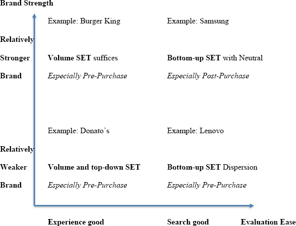
Conceptual framework.

Starting at the bottom left quadrant of Fig. 1, relatively weaker brands are less likely than relatively stronger brands to have been consumed by (most) readers of the social media post. Realizing this, social media posters are motivated to clearly express their liking or disliking of the brand to drive readers’ impression and purchase intent in the intended direction (Hoffman & Fodor, 2010). This should hold true especially for experience goods, i.e., goods that have to be experienced to readily evaluate their quality. Our rationale is analogous to that for construct clarity in Humphreys and Wang, 2017: “if the construct is relatively clear (e.g., positive affect), one can use dictionary or rule set to measure the construct” (p. 29). In these clear cases, top-down approaches have the dual advantage of easier implementation, especially for researchers with limited programming or coding experience, and easier operationalization of general constructs and theories directly from social science (Humphreys & Wang, 2017). Our example is Donato's, in our sample a relatively weaker brand in gastronomy/restaurant meals, a category high in experience qualities (Zeithaml, 1981). After purchase, the personal experience of the survey respondent should matter more than any opinion on social media; hence we posit that a bottom-up approach such as LIWC should be especially valuable in the pre-purchase stages.

In contrast, brands in search categories can be readily evaluated before purchase. For instance, the technical specifications and pictures of a Lenovo computer enable the potential customer (with some expertise in the computing category) to imagine the future experience with the product. Thus, social media posters can use positive words to steer consumers away from the brand (“@Delta Losing my bag is a great way to keep me as a customer”) or use negative words even in a positive review to elaborate on minor annoyances, such as “I was extremely irritated when it came in a giant box with no bubble wrap, only wrapped in Brown paper,” without risking to greatly decrease purchase intent by potential customers. As a result, we expect that bottom-up approaches are needed to subtly understand the nuances of sentiment for relatively weaker brands of search categories. Likewise, Humphreys and Wang (2017) recommend bottom-up approaches when “the operationalization of the construct in words is not yet clear or the researcher wants to make a posteriori discoveries about operationalization.” Even if most words in a sentence reflect positive sentiment in the dictionary, putting them together reflect the opposite: “@Delta Losing my bag is a great way to keep me as a customer.” This sarcasm is difficult to detect online and requires context to understand it (Morrison, 2016). Bottom-up approaches have the dual advantage of providing the likelihood of types and reveal new insights, “such as surprising combinations of words or patterns that may have been excluded in a top-down analysis” (Humphreys & Wang, 2017). To drive pre-purchase stages, such sentiment should have a clear directionality to even matter in the context of the readily available search attributes. Thus, we expect positive/negative comparisons to suffice, although neutral comments should still play a role.

Moving to relatively stronger brands in search categories, we posit that in this case the social media poster perceives maximum leeway to engage in irony, sarcasm and innuendos that require the most sophisticated SET to decipher. The difference between Neutral versus predominantly positive/ negative sentiment becomes important in this top right quadrant of Fig. 1. Our brand example is Samsung, for which a social media post reads “I'm so angry that the TV I surprised my beloved husband with for his birthday keeps turning off every three minutes!!!! This is terrific! And to make it even better, you guys know of the problem and have not corrected it!!!.” The high frequency of both positive and negative words requires more sophisticated SET with neutral comments.

Finally, relatively stronger brands in experience categories often aim to simply remind consumers about the experience and strive for volume in social media. For instance, for its 2019 Superbowl ad, Burger King anticipated that “half the conversation revolved around genuine confusion over [Warhol's] identity or what they'd just watched’ but chose the spot because it was immediately clear #EatLikeAndy had the ‘x factor’ consumers would talk, post, and tweet about on social.” Indeed, Colicev et al. (2018, p. 46) name Burger King as a company for which “negative-valence Earned Social Media (ESM) sometimes moves with Purchase Intent,” suggesting that “contrary to common wisdom, this would suggest that Burger King's performance is driven by Earned Social Media Engagement Volume (ENG) rather than negative-valence ESM.” We agree this version of “all publicity is good publicity” may well be the case in driving pre-purchase stages. As a result, volume metrics would suffice, and SETs classifying sentiment as positive or negative may not add much to the explanation of brand awareness, impression or purchase intent.

In sum, we have several expectations, as summarized in Fig. 1, but the picture is complicated by the many stages of the customer decision journey and potential contingency factors. For instance, the relative value of sentiment classification could well depend on whether average sentiment expressed in the industry is mostly negative or positive—a factor that cannot readily be assessed before applying the SETs. Therefore, we set out to estimate the explanatory power of each SET for each stage and to explore the impact of brand and category factors and their interactions in a contingency analysis, as detailed below.

Data

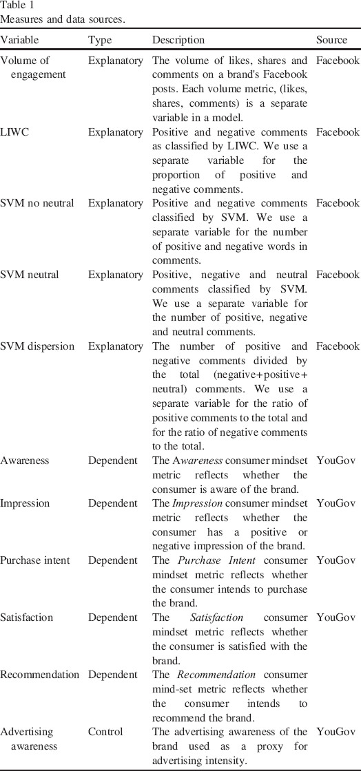
We construct our time series variables by merging two separate data sets that have observations collected for different time frequencies (see Table 1 for details on the data and variables). Social media data are obtained from each brand's official presence on Facebook. Consumer mindset metrics are collected from YouGov group and are available for a daily frequency. As social media data come at a high frequency (any point during a day), we aggregate social media data to the level of daily frequencies prior to merging the two data sets.

Table 1

Measures and data sources.

Variable	Type	Description	Source
Volume of engagement	Explanatory	The volume of likes, shares and comments on a brand's Facebook posts. Each volume metric, (likes, shares, comments) is a separate variable in a model.	Facebook
LIWC	Explanatory	Positive and negative comments as classified by LIWC. We use a separate variable for the proportion of positive and negative comments.	Facebook
SVM no neutral	Explanatory	Positive and negative comments classified by SVM. We use a separate variable for the number of positive and negative words in comments.	Facebook
SVM neutral	Explanatory	Positive, negative and neutral comments classified by SVM. We use a separate variable for the number of positive, negative and neutral comments.	Facebook
SVM dispersion	Explanatory	The number of positive and negative comments divided by the total (negative + positive + neutral) comments. We use a separate variable for the ratio of positive comments to the total and for the ratio of negative comments to the total.	Facebook
Awareness	Dependent	The Awareness consumer mindset metric reflects whether the consumer is aware of the brand.	YouGov
Impression	Dependent	The Impression consumer mindset metric reflects whether the consumer has a positive or negative impression of the brand.	YouGov
Purchase intent	Dependent	The Purchase Intent consumer mindset metric reflects whether the consumer intends to purchase the brand.	YouGov
Satisfaction	Dependent	The Satisfaction consumer mindset metric reflects whether the consumer is satisfied with the brand.	YouGov
Recommendation	Dependent	The Recommendation consumer mind-set metric reflects whether the consumer intends to recommend the brand.
Advertising awareness	Control	The advertising awareness of the brand used as a proxy for advertising intensity.	YouGov

We successfully obtained comprehensive data for the 8 industries (airlines, banking, beverages, cars, consumer electronics, fashion, food and gastronomy) and 48 brands listed in Table 2.

Table 2

Brand sample.

Industry classification (YouGov group*)	Brands
Airlines	American Airlines, Frontier, Jenn Air, JetBlue, Lufthansa, Qantas, Singapore Airlines, Southwest
Banking	Fidelity, Fifth Third, Huntington Bank, JPMorgan, Liberty Mutual PNC Bank, Rabobank, US Bank
Beverages	Dos Equis, Hennessy, Jack Daniels, Jameson, Smirnoff
Cars	Audi, BMW, Ford, Kia, Lexus, Subaru, Volkswagen, Volvo
Consumer electronics	Apple, Lenovo, Samsung, SanDisk, Sony
Fashion	Abercrombie & Fitch, Aeropostale, Nine West North Face, JosA Bank
Food	Kettle Brand Chips, Nestea, Pepsi, Tostitos
Gastronomy	Burger King, Donato's, Kona Grill, McDonalds, Starbucks Frappucino

*

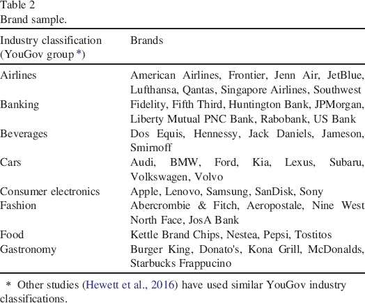
Other studies (Hewett et al., 2016) have used similar YouGov industry classifications.

Although all of the included brands have existed for a while, they differ in consumer awareness (e.g., 91% for American Airlines vs. 33% for Singapore Airlines according to YouGov), just as the industries differ in average sentiment (negative for airlines and banking while neutral or positive for the other industries). The final data set includes the period from November 2012 to June 2014, with 27,956 brand-day observations for the 48 unique brands.

Social Media Data

To collect social media data, we developed a crawler to extract all public information on the official Facebook page of each brand. Although future research may compare SETs on other platforms, Facebook is a good choice for maintaining the focus of the analysis on the same platform. As the largest social media platform, Facebook provides a dynamic environment for brand-consumer interactions. We collect more than 5 million comments on brand posts for our sample of brands and extract the sentiment from this textual data.

SET Application to Social Media Data

We collect classic pre-SET volume-based metrics with the help of Likes, Comments, and Shares of diverse Facebook content directly from Facebook's API. As the number of likes, comments and shares given to corporate posts on a company's Facebook page may also depend on the frequency a company posts, we additionally collect all posts from users on a company's Facebook page and count for these posts also the likes, comments, and shares.

We use the most frequent top-down approach available on the market: LIWC. LIWC provides word lists for 21 standard linguistic dimensions (e.g., affect words, personal concerns). To ensure a balanced set of sentiments we only use the general positive and negative sub-dimensions provided by LIWC. For each brand we export the extracted user posts and comments directly to LIWC that counts for each post and comment the number of positive and negative words and divides each by the number of total words per post or comment.

For our bottom-up approach, we collected 15 million context specific Amazon product reviews as training data. For each industry we construct context-specific training sets with reviews originating from each product category. To ensure that we only include very positive and very negative reviews, we further only rely on reviews with very low star rating (1) and very high star ratings (5). All other reviews are dropped from the training set. Then we proceed with standard NLP procedures as described in “Bottom-up Approaches”. For each product category we train a specific SVM. In addition, we collected for each category more 1- and 5-star reviews as a holdout sample (with 20% size of the training data). To test the accuracy of our category specific SVMs we predicted for the reviews in our hold out sample whether they were positive or negative. Hold out accuracies ranged from 80% to 92%, which we take a strong evidence that our SVMs have sufficient classification power. Web Appendix A and B provide details on brand sample composition, the training data and the hold out prediction accuracy.

To measure sentiment of user comments, we apply each trained category specific SVM to its corresponding user posts and comments. The trained SVM then classifies each post and comment to be either positive or negative. The SVM build into the RTextTool package further provides a classification likelihood for each post and comment. In case that a classification likelihood falls below 70% we follow Joshi and Tekchandani (2016) and believe the post or comment to be neither positive nor negative, but neutral and mark them correspondingly. We then aggregate sentiments by first building the daily sum for positive, negative and neutral comments, and further calculate the share of daily positive to total and negative to total comments, which we refer to as SVM Dispersion, a measure that is comparable to the top-down approaches’ relative sentiment measure that similarly divides the number of positive or negative words in a post or comment by the total number of words in this post or comment.

Consumer Mindset Metrics

We have access to a unique database from the market research company, YouGov group, which provides a nationwide measurement of daily consumer mindset metrics. Through its BrandIndex panel (http://www.brandindex.com), YouGov monitors multiple brands across industries by surveying 5,000 randomly selected consumers (from a panel of 5 million) on a daily basis. To assure representativeness, YouGov weighs the sample by age, race, gender, education, income, and region.

YouGov data have been previously used in the marketing literature (Colicev et al., 2018; Colicev, O'Connor, & Vinzi, 2016; Hewett, Rand, Rust, & van Heerde, 2016) and exhibit at least four advantages. First, such survey data are considered an appropriate analytical tool in marketing research (e.g., Steenkamp & Trijp, 1997) and have been shown to drive brand sales (Hanssens et al., 2014; Pauwels, Aksehirli, & Lackman, 2016; Srinivasan, Vanhuele, & Pauwels, 2010). Second, the YouGov panel has substantial validity, as it uses a large and diverse set of consumers that captures the “wisdom of the crowd” and between-subject variance. In recent comparisons with other online surveys, YouGov emerged as the most successful (FiveThirtyEight, 2016; MacLeod, 2012). Third, YouGov administers the same set of questions for each brand, which assures consistency for each metric, and, in any single survey, an individual is only asked about one measure for each industry; thus, reducing common method bias and measurement error. Finally, YouGov data are collected daily, thereby rapidly incorporating changes in consumer attitudes towards brands. As a result, YouGov data overcomes many of the normal limitations of using survey data, specifically the difficulty and expense of recruiting a sufficient number of participants and the challenges of low frequency and outdated data (Steenkamp & Trijp, 1997).

We use five common mindset metrics that capture the consumer purchase funnel/decision journey: awareness, impression, purchase intent, satisfaction and recommendation (details on the exact items and data collection are provided in Web Appendix C). “Awareness” reflects general brand awareness, “impression” captures brand image, “purchase intent” indicates purchasing intentions, “satisfaction” captures general satisfaction with the brand, and “recommendation” captures brand referrals. Given its importance in prior literature (Srinivasan, Vanhuele, & Pauwels, 2010), we also include a control variable, YouGov's metric, “Advertising Awareness,” as a proxy for brands’ advertising expenditures. At the aggregate brand level, the scores on the measures from YouGov fall within the range of − 100 to + 100. For customer satisfaction, as an example, the extremes are only realized when all respondents agree in their negative or positive perception of the brand relative to its competitors. The daily measures of mindset metrics are based on a large sample of 5,000 responses; this approach helps to reduce sampling error.

Method

Overview of the Approach

As depicted in Fig. 2, our analysis consists of a set of several methodological steps.

Fig. 2

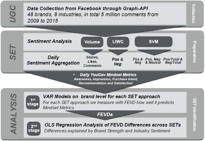
Overview of data and analysis.

Our choice of econometric model is driven by the criteria that it can (1) account for the possibly dynamic nature and dual causality of the relations between SET metrics and the various consumer mindset metrics and (2) uncover which form of SET best explains consumers’ mindset over time for each brand (whose time period of data availability may not completely overlap with that of other brands). Therefore, we estimate a vector autoregressive (VAR) model per brand (Colicev et al., 2018; Ilhan, Kübler, & Pauwels, 2018). VAR accounts for the potential endogeneity between social media and consumer mindset metrics while controlling for the effects of exogenous variables that could potentially affect both metrics (e.g., advertising). In addition, VAR provides a measure of the relative impact of shocks that are initiated by each of the individual endogenous variables in a model through forecast error variance decomposition (FEVD). This measure allows us to compare the relative performance of different SETs for the explained variance in consumer mindset metrics (Srinivasan, Vanhuele, & Pauwels, 2010).

For the sentiment variables, we have five different SETs to assess sentiment: (1) the Volume (number) of likes, comments and shares of brand posts, and, for the comments, the sentiment analysis of (2) LIWC, (3) SVM (without the neutral sentiment comments), (4) SVM Dispersion (adjusted for sentiment dispersion), and (5) SVM Neutral (with the neutral sentiment comments). We estimate a separate VAR model for each brand that relates one SET at a time to five mindset metrics: awareness, impression, purchase intent, satisfaction and recommendation. We also estimate SET combinations in Models 6–9, with Model 6 combining Volume and SVM Neutral, Model 7 Volume and LIWC, Model 8 LIWC and SVM Neutral and Model 9 Volume, LIWC and SVM Neutral. Finally, we check the per-metric performance and combine them into a unifying model, Model 10. Thus, in total, we estimate 10 different models for each of the 48 brands, which results in 480 VAR models.

To evaluate how each SET explains the dynamic variation in each mindset metric for each brand, we use FEVD, as in Srinivasan, Vanhuele, and Pauwels (2010). Next, we aggregate the FEVD across all five consumer mindset metrics to form an aggregated measure of performance of the SETs across both brands and mindset metrics. Thus, in this step, we can assess (a) the performance of SETs individually for each brand and (b) the performance of SETs aggregated across all brands.

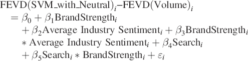
In the second step, we use the brand-level FEVD scores in a second-stage regression to establish the brand and industry characteristics that can explain the relative performance (FEVD) of SETs. Our dependent variable is the relative quality scores for each brand and each SET, computed by subtracting the FEVD for each SET from the FEVD of the most sophisticated SET (SVM Neutral). In total, we have four quality scores that consist of the difference in the FEVD between the SVM Neutral and the other SETs (1) the Volume measures, (2) SVM without a neutral option, (3) LIWC and (4) SVM with dispersion. These relative quality scores are regressed on brand strength, average industry sentiment, the search (vs. experience) good nature of the category, and the interaction of each category variable with brand strength. Thus, we run a total of 20 s-stage regressions (4 FEVD comparisons times five mindset metrics), which each have 48 data points (the number of brands).

We compute the brand strength as the average of the studied mindset metrics over our period of investigation. For example, when the quality score that was mentioned above is assessed for the explanatory power of the awareness mindset metric, we use the average awareness score for the brands over the investigation period. We note that our sample is mostly composed of strong brands and thus our brand strength metric is relative. For industry sentiment, we compute the average industry sentiment for each industry over the investigation period. This results in a measure that reflects whether the sentiment in the industry is more negative (e.g., banks) or positive (e.g., fashion). For search/experience nature of the category we split the sample into search (airlines, beverages, consumer electronics and clothes) and experience categories (banking, cars, food and gastronomy) – following the taxonomy in Zeithaml (1981).

Econometric Model Specification

Based on the unit root tests, we specify a VAR in levels for each brand/SET combination. Eq. (1) shows the specification for SET Volume, which is captured by three variables: number of likes, comments and shares:

$$\left[\begin{array}{c}{\text{Likes}}_{\mathrm{t}}\\ {\text{Comments}}_{\mathrm{t}}\\ {\text{Shares}}_{\mathrm{t}}\\ {\text{Awareness}}_{\mathrm{t}}\\ {\text{Impression}}_{\mathrm{t}}\\ {\text{Purchase Intent}}_{\mathrm{t}}\\ {\text{Satisfaction}}_{\mathrm{t}}\\ {\text{Recommendation}}_{\mathrm{t}}\end{array}\right]=\sum _{\mathrm{n}=1}^{\mathrm{p}}\left[\begin{array}{ccc}{\mathrm{\gamma }}_{1,1}^{\mathrm{n}}& .& {\mathrm{\gamma }}_{1,8}^{\mathrm{n}}\\ .& .& .\\ {\mathrm{\gamma }}_{8,1}^{\mathrm{n}}& .& {\mathrm{\gamma }}_{8,8}^{\mathrm{n}}\end{array}\right]\left[\begin{array}{c}{\text{Likes}}_{\mathrm{t}-\mathrm{n}}\\ {\text{Comments}}_{\mathrm{t}-\mathrm{n}}\\ {\text{Shares}}_{\mathrm{t}-\mathrm{n}}\\ {\text{Awareness}}_{\mathrm{t}-\mathrm{n}}\\ {\text{Impression}}_{\mathrm{t}-\mathrm{n}}\\ {\text{Purchase Intent}}_{\mathrm{t}-\mathrm{n}}\\ {\text{Satisfaction}}_{\mathrm{t}-\mathrm{n}}\\ {\text{Recommendation}}_{\mathrm{t}-\mathrm{n}}\end{array}\right]+\left[\begin{array}{ccc}{\mathrm{\phi }}_{1,1}& .& {\mathrm{\phi }}_{1,2}\\ .& .& .\\ {\mathrm{\phi }}_{8,1}& .& {\mathrm{\phi }}_{8,2}\end{array}\right]\left[\begin{array}{c}{\mathrm{x}}_1\\ {\mathrm{x}}_2\end{array}\right]+\left[\begin{array}{c}{e}_{1\mathrm{t}}\\ e_{2\mathrm{t}}\\ e_{3\mathrm{t}}\\ e_{4\mathrm{t}}\\ \begin{array}{c}{e}_{5\mathrm{t}}\\ e_{6\mathrm{t}}\\ e_{7\mathrm{t}}\\ e_{8\mathrm{t}}\end{array}\end{array}\right]$$

(1)where for each day t, likes = Volume metric of likes, comments = Volume metric of comments, shares = Volume metric of shares, awareness = Awareness mindset metric, impression = Impression mindset metric, purchase = Purchase intent mindset metric, satisfaction = Customer Satisfaction mindset metric, and recommendation = Recommendation mindset metric. This vector of endogenous variables is regressed on its past for p days, with the lag p chosen to balance the model parsimony with forecasting accuracy. We begin with the optimal lag p according to the Akaike Information Criterion (AIC) and then check whether we should add lags based on diagnostic tests for residual autocorrelation (Franses, 2005). The vector of exogenous variables (verified as such with Granger causality tests) contains the Advertising Awareness (x ₁ ) variable and a deterministic trend t (x ₂ ) to reflect the impact of omitted, gradually changing influences. Finally, the forecast errors, ε, have a full variance–covariance matrix, Ω, allowing for examining the same-day effects of one endogenous variable on another.

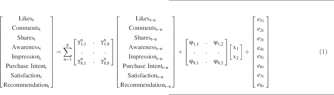
For the model specification for the other SETs, we replace the three volume metrics in Eq. (1) with the corresponding metrics in the SET. In this respect, Model 2 has SVM without neutral comments, Model 3 LIWC, Model 4 SVM Dispersion, Model 5 SVM with neutral comments. Then, we combine different SETs in the same model estimation. Accordingly, Model 6 has Volume and SVM Neutral (6 variables), Model 7 Volume and LIWC (5 variables), Model 8 LIWC and SVM Neutral (5 variables), Model 9 Volume and LIWC and SVM Neutral (8 variables) and Model 10 Best predictive combination of three variables.

Note that the SETs Volume (Model 1) and SVM Neutral (Model 5) have 3, while the others have 2 variables. A larger number of variables typically implies an advantage for in-sample fit (R2 and FEVD) and a disadvantage for out-of-sample predictions (Armstrong, 2001). Thus, we also display the FEVD results of the model after dividing by the number of variables. Please refer to Web Appendix D for details on model specification.

Impulse Response Functions (IRF) and Forecast Error Variance Decomposition (FEVD)

From the VAR estimates, we derive the two typical outputs of IRFs; tracking the over-time effect of a 1 unit change to a SET metric on the attitude of interest; and the attitude's FEVD, i.e., the extent to which it is dynamically explained by each SET metric (see Colicev, Kumar, & O'Connor 2019). To obtain prototypes of IRFs that account for similar and consistent patterns across companies and contexts, we use a shape-based time series clustering approach that highlights an average, centroid IRF for each identified cluster (for more details see Mori, Mendiburu, & Lozano, 2016). While IRFs are not central to our study, they still provide a good metric on the direction and significance of the effects of SETs on mindset metrics.

The central metric for our study is the FEVD which allows us to compare the variance explained by each SETs in each mindset metric. First, FEVDs fit well with the purpose of the study which is to generate comparative results across SETs and mindset metrics. Second, previous research has used FEVD for similar purposes (see for e.g., Srinivasan, Vanhuele, & Pauwels, 2010 where they compare the explanatory power of different metrics). Third, FEVDs also allow us to abstain from directions of the effects (as in IRFs) and focus on explanatory power over time. Indeed, we evaluate FEVDs at 30 days to reduce sensitivity to short-term fluctuations.

We use the Cholesky ordering based on the results from the Granger causality tests to impose a causal ordering of the variables. To prevent the effects of this ordering on the results, we rotate the order of the endogenous variables and compute averages over the different responses as a consequence of one standard deviation shocks (e.g., Dekimpe & Hanssens, 1995). To assess the statistical significance of the FEVD estimates, we obtain standard errors using Monte Carlo simulations with 1,000 runs (Nijs, Srinivasan, & Pauwels, 2007). For each SET, we sum the variance of its metrics to calculate the total percentage of the mindset metric that is explained by the SET. Moreover, as some SETs have more variables than others, we also calculate and compare the FEVD per SET variable.

Second-Stage Regressions

In Eq. (2) below, we show the second-stage estimation for the difference between SVM Neutral (best performing SET) and Volume metrics for each consumer mindset metric:

$$\begin{array}{l}FEVD{\left(SVM\_with\_Neutral\right)}_i-FEVD{\left(Volume\right)}_i\\ \hspace{0.17em}\hspace{0.17em}\hspace{0.17em}={\beta }_0+{\beta }_{1}BrandStrengt{\text{h}}_i\\ \hspace{0.17em}\hspace{0.17em}\hspace{0.17em}\hspace{0.17em}\hspace{0.17em}+{\beta }_{2}AverageIndustrySentimen{\text{t}}_i+{\beta }_{3}BrandStrengt{\text{h}}_i\\ \hspace{0.17em}\hspace{0.17em}\hspace{0.17em}\hspace{0.17em}\hspace{0.17em}*AverageIndustrySentimen{\text{t}}_i+{\beta }_{4}Searc{h}_i\\ \hspace{0.17em}\hspace{0.17em}\hspace{0.17em}\hspace{0.17em}\hspace{0.17em}+{\beta }_{5}Searc{h}_i*BrandStrengt{\text{h}}_i+{\epsilon }_i\end{array}$$

(2)where FEVD(SVM_with_Neutral) = variance explained in the consumer mindset metric by the positive, negative and neutral comments that were extracted by SVM; FEVD(Volume) = variance explained in the consumer mindset metric by likes, shares and comments; FEVD(SVM) = variance explained in the consumer mindset metric by positive and negative comments that were extracted by SVM; FEVD(LIWC) = variance explained in the consumer mindset metric by positive and negative comments that were extracted by LIWC; and FEVD(SVM_Dispersion) = variance explained in the consumer mindset metric by positive and negative comments that were extracted by SVM and adjusted for dispersion. At explanatory variables, we include the main effects of brand strength (β₁) average industry sentiment (β₂), the search (vs. experience) good nature of the category (β₄), and the interaction of each category variable with the brand strength variable (β₃, β₅). For example, a positive β₁ coefficient would imply that SVM Neutral would have a higher explanatory power with respect to the compared metric (e.g., Volume in quality score 1 as in the example above). As coefficients are standardized, the coefficient should be interpreted as the effects of one standard deviation increase in brand strength in affecting FEVD difference by a certain percentage. In addition, a negative β₅ coefficient would suggest that for relatively stronger brands in search goods category would benefit from Volume in contrast to SVM Neutral (for quality score 1). Fashion is a search product with negative industry sentiment, while airlines, electronics and beverages enjoy positive industry sentiment. For experience products, banking, and food have negative average sentiment while cars and gastronomy enjoy positive sentiment.

Results

Descriptive Statistics

In Table 3, we present the correlations among the variables (averaged across brands).

Table 3

Correlations among model variables (average across brands and SET variables).

	Likes (Volume)	Comments (Volume)	Shares (Volume)	Negative (SVM)	Positive (SVM)	Neutral (SVM)	Positive (LIWC)	Negative (LIWC)	Positive (SVM Dispersion)	Negative (SVM Dispersion)	Awareness	Impression	Purchase Intent	Recommendation	Satisfaction
Likes (volume)	1.000
Comments (volume)	0.594	1.000
Shares (volume)	0.767	0.552	1.000
SVM (negative)	0.260	0.460	0.241	1.000
SVM (positive)	0.350	0.595	0.331	0.589	1.000
SVM (neutral)	0.309	0.616	0.300	0.696	0.718	1.000
LIWC (positive)	0.382	0.541	0.363	0.583	0.767	0.742	1.000
LIWC (negative)	0.227	0.406	0.237	0.620	0.571	0.627	0.578	1.000
SVM Dispersion (positive)	0.101	0.070	0.082	− 0.066	0.242	− 0.036	0.124	0.009	1.000
SVM dispersion (negative)	− 0.020	− 0.021	− 0.016	0.291	− 0.039	− 0.013	− 0.027	0.053	− 0.256	1.000
Awareness	− 0.003	0.003	− 0.001	0.010	0.007	0.001	0.006	0.001	− 0.011	0.013	1.000
Impression	0.004	0.008	0.003	− 0.002	0.002	− 0.002	0.004	− 0.007	− 0.004	0.003	0.203	1.000
Purchase intent	0.008	0.001	0.009	0.007	0.005	0.009	0.004	0.003	− 0.001	0.009	0.135	0.240	1.000
Recommendation	0.008	0.005	0.005	− 0.006	− 0.004	− 0.004	− 0.002	− 0.010	− 0.002	− 0.004	0.155	0.634	0.243	1.000
Satisfaction	0.019	0.014	0.011	− 0.001	0.011	0.013	0.013	0.002	0.011	− 0.007	0.171	0.470	0.307	0.471	1.000

First, the volume and sentiment variables have a moderate correlation with the mindset metrics, with the strongest correlation being between satisfaction and volume (0.019). This reflects previous research that online sentiment does not fully overlap with mindset metrics in the broader consumer population (Baker, Donthu, & Kumar, 2016; Lovett, Peres, & Shachar, 2013; Ruths & Pfeffer, 2014). The correlation among SET metrics is higher (up to 0.767 for LIWC positive and SVM positive) but not perfect, which highlights the importance of researchers’ SET choice. Finally, the correlations among the pre-purchase mindset metrics is moderate (0.14–0.24), which reflects their divergent validity. Naturally, the post-purchase metrics satisfaction and recommendation have a higher correlation.

VAR Model Fit and Lag Selection

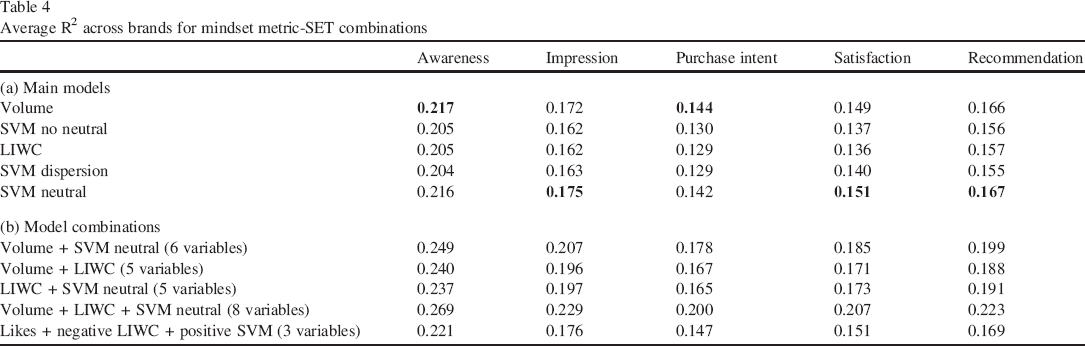
All VAR models passed the tests for descriptive models according to Franses (2005), and the SETs explained between 13% and 22% of the daily variation (R²) for each mindset metric (Table 4). As expected, SETs have a tougher time explaining purchase intent than awareness. As shown in Table 4a, SVM Neutral and Volume have the highest average R² across all mindset metrics. Table 4b shows how explanatory power improves by combining different SETs, with the Model 9 combination (volume metrics + LIWC + SVM with neutral) explaining at least 20% of each mindset metric. All brand level-results are available in Web Appendix E.

Table 4

Average R² across brands for mindset metric-SET combinations

	Awareness	Impression	Purchase intent	Satisfaction	Recommendation
(a) Main models
Volume	0.217	0.172	0.144	0.149	0.166
SVM no neutral	0.205	0.162	0.130	0.137	0.156
LIWC	0.205	0.162	0.129	0.136	0.157
SVM dispersion	0.204	0.163	0.129	0.140	0.155
SVM neutral	0.216	0.175	0.142	0.151	0.167
(b) Model combinations
Volume + SVM neutral (6 variables)	0.249	0.207	0.178	0.185	0.199
Volume + LIWC (5 variables)	0.240	0.196	0.167	0.171	0.188
LIWC + SVM neutral (5 variables)	0.237	0.197	0.165	0.173	0.191
Volume + LIWC + SVM neutral (8 variables)	0.269	0.229	0.200	0.207	0.223
Likes + negative LIWC + positive SVM (3 variables)	0.221	0.176	0.147	0.151	0.169

The Impact of SET Metrics on Consumer Mindset Metrics: Impulse Response Functions

The IRFs show that all effects of SET metrics on consumer attitudes stabilize within a month, most within 10 days. As an illustration, Fig. 3 contrasts the impact of volume metric Likes with that positive top-down (LIWC) on each consumer attitude for the major clusters.

Fig. 3

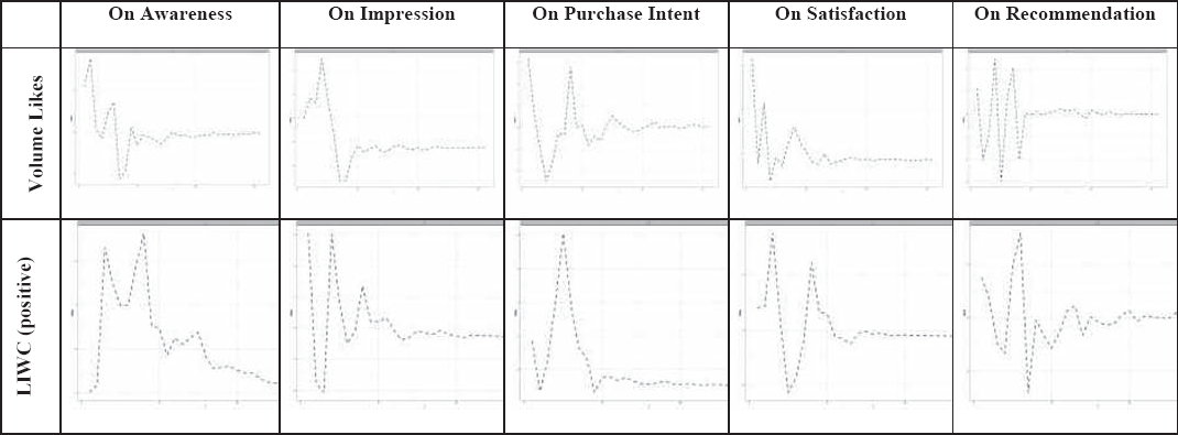
Impulse response functions of sentiment extraction metrics on attitudes.

For first four of stages Awareness, Impression, Purchase Intent and Satisfaction, Likes have a strong initial effect and a fairly typical decay pattern. In contrast, the effect on Recommendation oscillates wildly from first day, indicating that Likes have little explanatory power for this post-purchase stage (as verified in the FEVD). Meanwhile, positive sentiment (as classified by LIWC) shows the typical over-time impact on Recommendation. Across consumer attitude metrics, the peak impact of positive LIWC sentiment occurs later than the peak impact of Likes. This points to the key importance of assessing dynamic explanation, as we do in the FEVD comparison.

Relative Importance of Metrics: Forecast Error Variance Decomposition (FEVD)

We aggregate the results across brands in Table 5.

Table 5

FEVD results for main models.

	Variance decomposition of
SETs	Awareness	Impression	Purchase Intent	Satisfaction	Recommendation
(a) FEVD of the mindset metric: Results for 5 main models
Volume (SUM of its metrics)	5.17	4.44	4.55	4.10	4.19
SVM (SUM)	3.63	3.07	2.68	2.74	2.93
LIWC (SUM)	3.41	3.08	2.71	2.65	3.00
SVM dispersion (SUM)	3.47	3.34	2.83	3.02	2.95
SVM neutral (SUM)	5.13	4.60	4.15	4.27	4.31
(b) FEVD of the mindset metric: Results for the combined models
Volume + SVM neutral	9.68	8.82	8.51	8.55	8.47
Volume + LIWC	8.15	7.42	7.14	6.93	7.05
LIWC + SVM neutral	7.80	7.41	6.93	6.94	7.21
Volume + LIWC + SVM neutral	12.38	11.76	11.47	11.67	11.31
Likes + negative LIWC (negative) + positive SVM	5.54	4.87	4.38	4.45	4.66

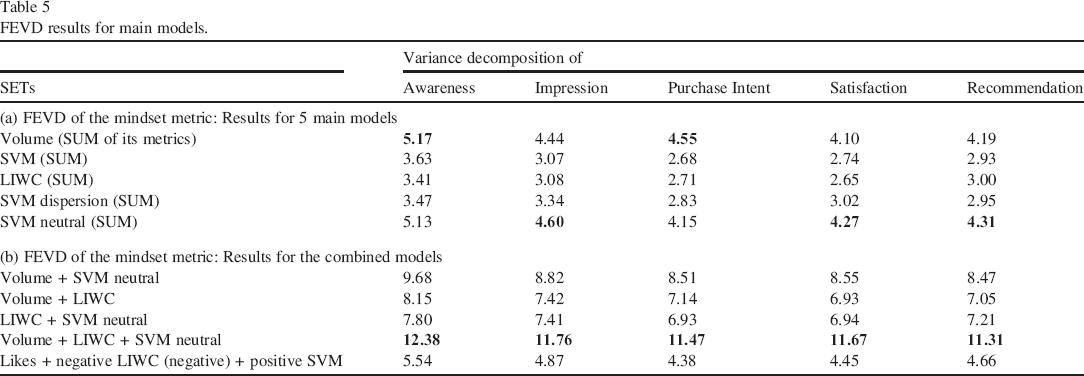
Across all analyzed brands, we find that SET Volume and SVM Neutral have the highest FEVD for all mindset metrics. SVM Dispersion performs well for impression, and LIWC for recommendation. These findings indicate that contingency factors may affect the explanatory power of SETs. For the combination of SET models, Table 5b shows that Model 9 (Volume + LIWC + SVM Neutral) obtains the highest averaged FEVD across brands. Table 6 further provides a summary of our main findings for each mindset metric and industry highlighting that different SETs might be suitable for different industries and metrics.

Table 6

Summary of the main findings.

	Awareness	Impression	Purchase intent	Satisfaction	Recommend
Aggregated results across all brands	Volume	SVM neutral	Volume	SVM neutral	SVM neutral
Brand results (number of brands for which SET explained most)	SVM neutral = 22	SVM neutral = 21	SVM neutral = 18	SVM neutral = 20	SVM neutral = 20
	Volume = 20	Volume = 19	Volume = 26	Volume = 21	Volume = 21
	SVM dispersion = 3	SVM dispersion = 4	SVM dispersion = 4	SVM dispersion = 5	SVM dispersion = 6
	LIWC = 3	LIWC = 4	LIWC = 0	LIWC = 2	LIWC = 1
	SVM no neutral = 0	SVM no neutral = 0	SVM no eutral = 0	SVM no neutral = 0	SVM no neutral = 0
Industry results	Awareness	Impression	Purchase intent	Satisfaction	Recommend
Airlines	Volume	SVM dispersion	No systematic difference	SVM neutral	SVM dispersion
Banking	Volume	Volume	No systematic difference	No systematic difference	SVM dispersion
Beverages	SVM dispersion	SVM dispersion	SVM dispersion	SVM dispersion	SVM dispersion
Cars	SVM dispersion	No systematic difference	No systematic difference	No systematic difference	No systematic difference
Electronics	SVM dispersion	SVM dispersion	SVM dispersion	SVM dispersion	SVM dispersion
Fashion	Volume	SVM neutral	Volume	Volume	SVM neutral
Food	SVM neutral	No systematic difference	No systematic difference	Volume	SVM neutral
Gastronomy	Volume	No systematic difference	SVM dispersion	No systematic difference	No systematic difference

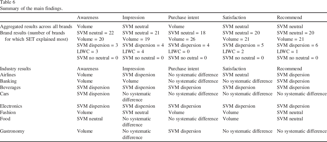
Beyond these average results, we observe heterogeneity across brands for which SETs explain the most variance. For example, for awareness, SVM Neutral has the highest explanatory power for 22 brands, Volume for 20 brands, SVM Dispersion for three brands and LIWC for three brands. Therefore, we further investigate the results by (1) relating them to brand and industry factors in our second stage and (2) reporting them by industry.

Second-Stage Analysis

The coefficient estimates and standard errors for the second-stage analysis are shown in Table 7.

Table 7

Second-stage regressions of forecast error variance decompositions (FEVD).

SVM Neutral's FEVD versus FEVD of:	Volume	SVM no neutral	LIWC	SVM dispersion
	Awareness
Brand strength	− 0.19706	− 0.05822	0.16491	0.35238
	(1.28)	(0.31)	(2.02)**	(2.77)***
Average industry sentiment	0.03802	0.14818	− 0.03463	− 0.38266
	(0.55)	(1.27)	(0.80)	(3.02)***
Industry sentiment × Brand strength	− 0.13167	− 0.02001	0.18380	− 0.09740
	(0.91)	(0.17)	(1.53)	(0.93)
Search good dummy (1 = search)	0.57942	0.02806	0.46013	0.15860
	(2.57)***	(0.12)	(1.86)	(0.63)
Search good dummy × Brand strength	0.21930	0.05937	− 0.06975	− 0.25651
	(0.84)	(0.16)	(0.36)	(1.26)
	Impression
Brand strength	− 0.02036	− 0.12311	0.33129	0.31102
	(0.08)	(0.87)	(2.57)***	(1.38)
Average industry sentiment	0.03397	0.23941	− 0.19745	− 0.18216
	(0.29)	(1.53)	(1.72)	(1.42)
Industry sentiment × Brand strength	0.00289	0.29041	0.21029	− 0.05081
	(0.01)	(3.76)***	(1.30)	(0.35)
Search good dummy (1 = search)	0.66273	0.18337	0.85588	0.30429
	(2.76)***	(0.64)	(6.10)***	(1.03)
Search good dummy × Brand strength	− 0.24666	− 0.00415	− 0.69057	− 0.28830
	(0.60)	(0.02)	(3.48)***	(0.87)
	Purchase intent
Brand strength	− 0.41865	− 0.77836	− 0.38381	− 0.68825
	(3.42)***	(2.42)***	(3.06)***	(6.37)***
Average industry sentiment	− 0.17950	− 0.20846	− 0.11437	0.07191
	(1.82)	(2.93)***	(2.23)**	(1.09)
Industry sentiment × Brand strength	− 0.04854	0.02187	− 0.09071	− 0.15021
	(0.27)	(0.11)	(1.06)	(1.31)
Search Good dummy (1 = search)	− 0.40746	− 0.26344	0.05653	− 0.42650
	(2.59)***	(2.69)***	(0.43)	(2.16)**
Search Good dummy × Brand Strength	0.42941	0.94330	0.45406	0.67417
	(2.23)**	(4.42)***	(4.50)***	(5.66)***
	Satisfaction
Brand strength	− 0.50449	− 0.32598	− 0.13555	− 0.12753
	(3.91)***	(2.90)***	(1.23)	(1.00)
Average industry sentiment	− 0.12514	− 0.15129	− 0.11026	− 0.24108
	(2.25)**	(2.88)***	(0.94)	(6.86)***
Industry sentiment × Brand strength	− 0.18354	− 0.11359	− 0.06290	− 0.29192
	(0.91)	(0.64)	(0.32)	(1.36)
Search good dummy (1 = search)	0.68940	0.74356	0.69640	0.78795
	(6.47)***	(4.39)***	(3.94)***	(5.52)***
Search good dummy × Brand strength	0.45762	0.29965	0.06545	− 0.00393
	(1.59)	(1.17)	(0.27)	(0.01)
	Recommendation
Brand strength	0.14099	0.22796	0.16492	0.45979
	(2.14)**	(2.02)**	(2.11)**	(2.51)***
Average industry sentiment	− 0.18850	0.03984	− 0.15969	− 0.12300
	(3.28)***	(0.26)	(2.21)**	(1.64)
Industry sentiment × Brand strength	0.06103	0.07101	0.06877	− 0.09382
	(1.08)	(1.11)	(0.99)	(0.84)
Search good dummy (1 = search)	0.93713	0.45866	0.94639	0.44934
	(5.93)***	(1.57)	(4.99)***	(2.24)**
Search good dummy × Brand strength	− 0.50982	− 0.24771	− 0.35451	− 0.53877
	(4.25)***	(1.51)	(3.57)***	(3.01)***

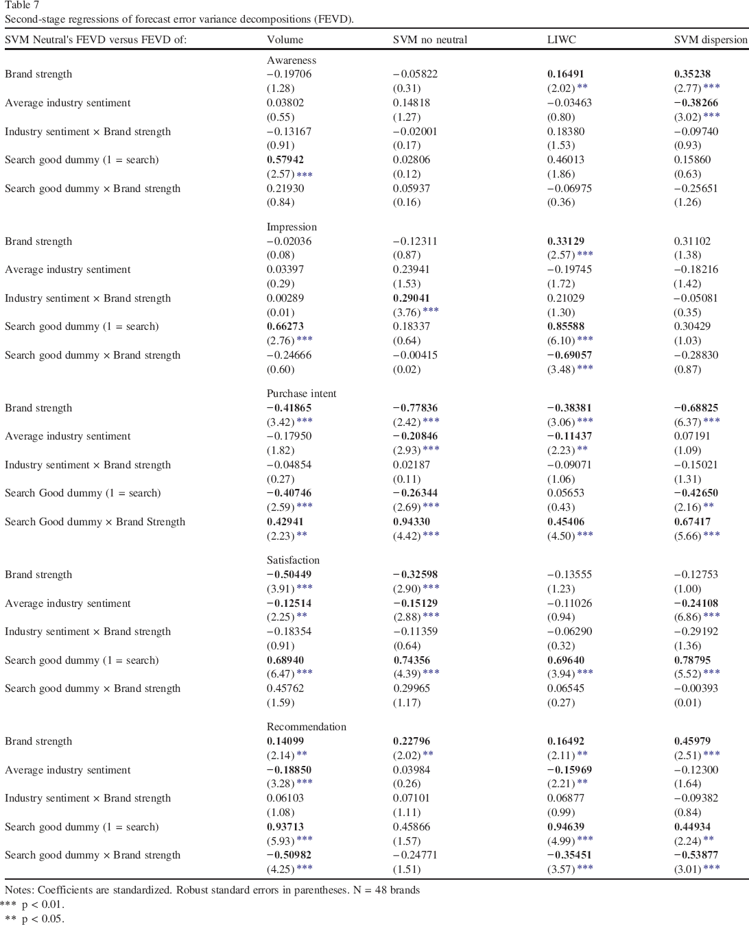
Notes: Coefficients are standardized. Robust standard errors in parentheses. N = 48 brands

***

p < 0.01.

**

p < 0.05.

The results vary across the four quality difference scores and mindset metrics, thus enhancing the ability to predict tactical decisions for the advantage of various SETs. Brand Strength and the Search/Experience nature of the category appear as the most important moderators for the explanatory power of SVM Neutral over alternatives. As to the former, relatively stronger brands see higher benefits than relatively weaker brands in using SVM Neutral to explain:

1. (1)

Awareness over LIWC (0.16, p < 0.05) and SVM dispersion (0.35, p < 0.05);

(2)

Impression over LIWC (0.33, p < 0.05);

(3)

Recommendation over all SET alternatives (0.14, 0.23, 0.16 and 0.46, respectively).

In contrast, relatively weaker brands see higher benefits than relatively stronger brands in using SVM Neutral to explain Purchase Intention over all SET alternatives and Satisfaction over Volume and SVM No Neutral. Thus, relatively weaker brands should spend their resources on more elaborate SET tools (such as SVM Neutral) when they are primarily interested in purchase-related attitudes.

As to the nature of the category, SVM Neutral has a higher explanatory power over alternative SETs for search goods versus experience goods for 4 out of 5 mindset metrics. First, SVM Neutral has better explanatory power than Volume (Column 2 of Table 7) for search goods when explaining Awareness, Impression, Satisfaction and Recommendation. Second, SVM Neutral has better explanatory power than SVM without neutral (Column 3 of Table 7) for search goods when explaining Satisfaction. However, experience goods are better off using SVM without neutral for purchase intent. Third, for SVM Neutral vs. LIWC (Column 4 of Table 7), the search good dummy has a significant positive coefficient for Impression, Satisfaction and Recommendation. Fourth, for SVM Neutral vs. SVM dispersion (Column 5 of Table 7), the search good dummy has a significant positive coefficient for Satisfaction and Recommendation, but a negative coefficient for purchase intent. Thus, managers of experience goods should pay special attention to sophisticated SETs when aiming to explain Purchase Intent.

When industry sentiment is low, we observe a higher benefit of SVM Neutral over SVM Dispersion for Awareness (− 0.38, p < 0.05), over SVM No Neutral and LIWC for Purchase Intent, over Volume, SVM No Neutral and SVM Dispersion for Satisfaction, and over Volume and LIWC for Recommendation. This consistent direction (no positive effects) indicates that it is especially crucial use bottom-up approaches and analyze Neutral comments when consumers typically complain about the product, as in airlines and banks versus fashion (e.g. Pauwels, Aksehirli, & Lackman, 2016). We speculate that it is simply harder to find positive signals among the many complaints, sarcasm and innuendos.

Interaction effects of brand strength and industry sentiment are significant for Impression, showing a higher benefit of SVM Neutral over SVM No Neutral when both the brand and industry sentiment are high. As before, we believe the preponderance of, in this case, positive comments, increases the importance of adding the Neutral comments to the analysis of impression. Finally, the interaction of brand strength and the nature of the product is significant for eight cases, which prompted us to visualize the main results in Fig. 4 (Purchase Intent) and Fig. 5 (Recommendation).

Fig. 4

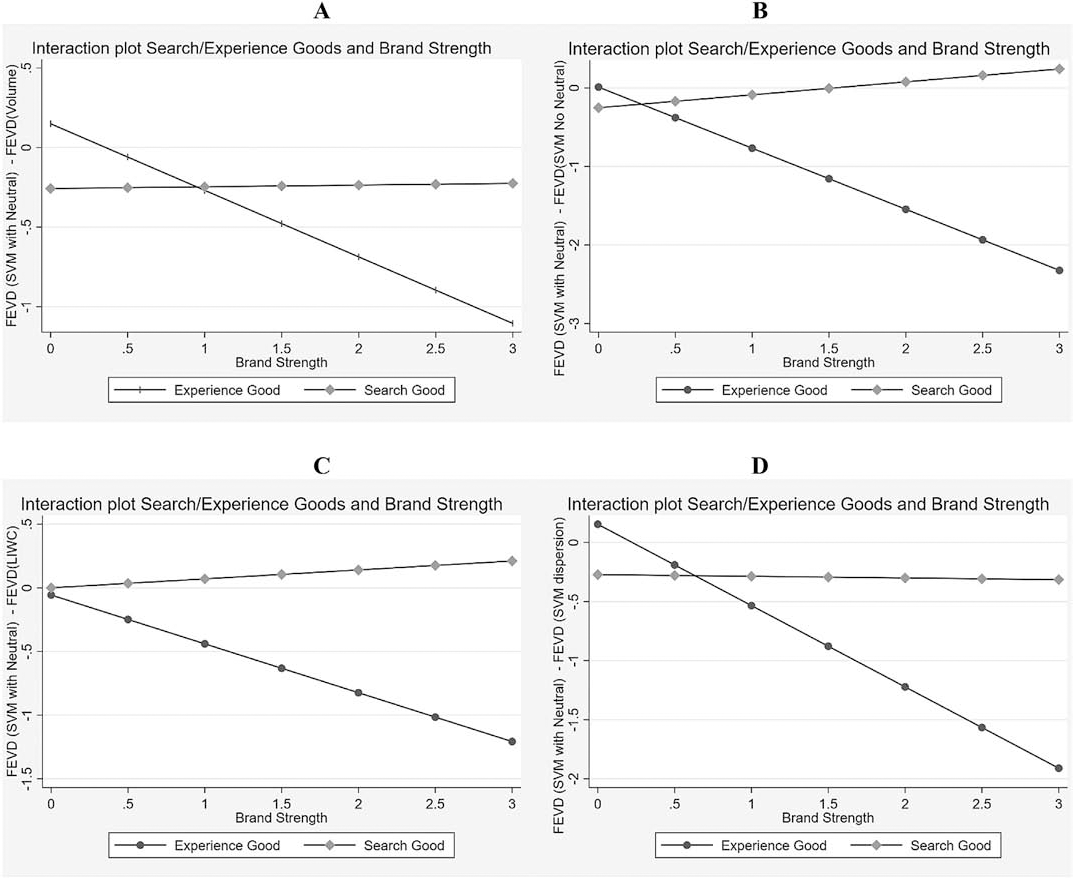
Interaction plots of the second-stage regression. Purchase intent.

Fig. 5

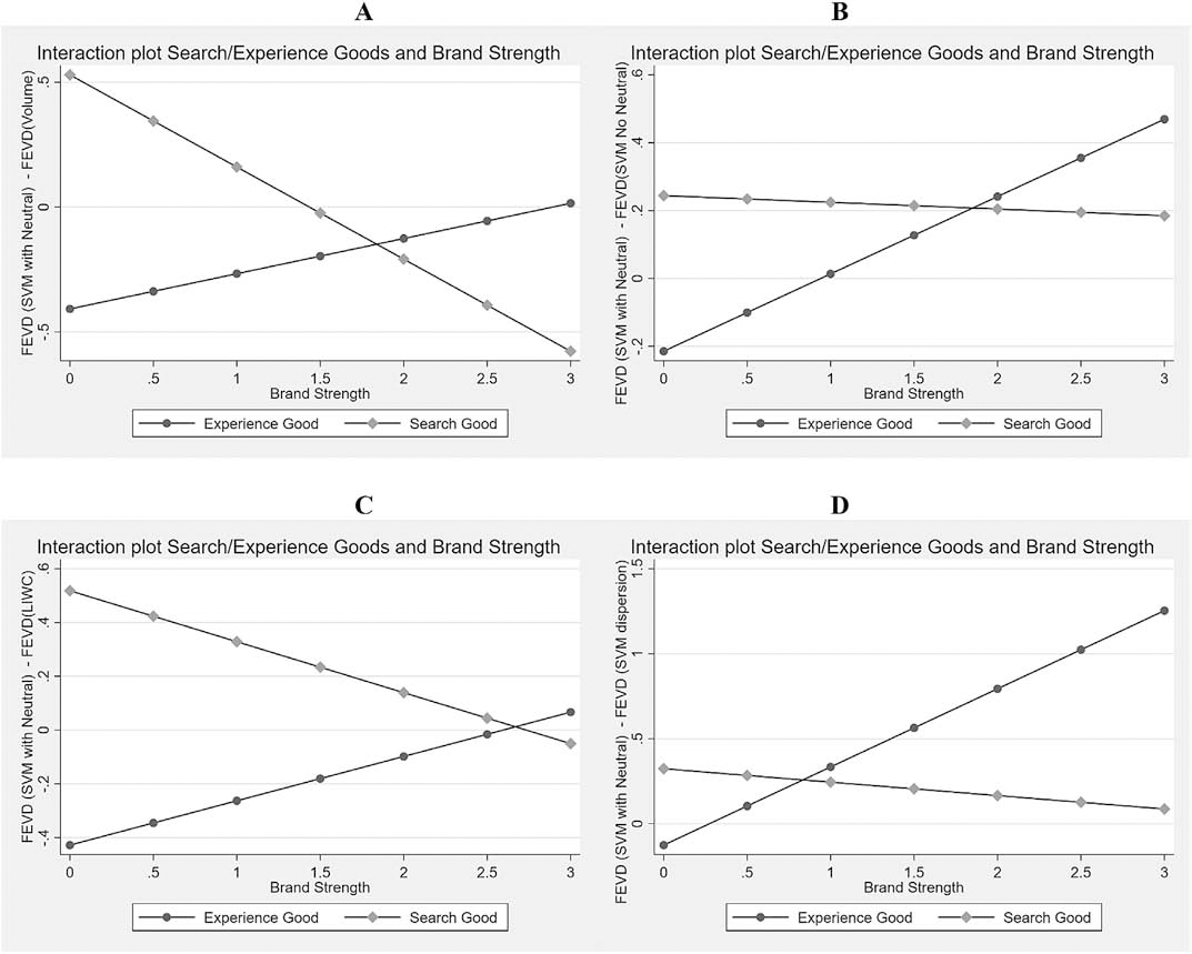
Interaction plots of the second-stage regression. Recommendations.

For purchase intent, results indicate that relatively stronger brands of experience goods should not use SVM No Neutral as their SET. In contrast, SVM No Neutral dominates over other alternatives for relatively weaker brands of experience goods and for stronger brands of search goods. For example, Panel 3A shows that SVM Neutral improves over Volume only for relatively weaker brands of experience goods. Panel 3B shows that SVM Neutral dominates SVM No Neutral for strong brands of search goods. Panel 3C shows the dominance of LIWC over SVM Neutral for Experience goods, especially when the brand is strong. For Recommendation, panel 4A shows a higher benefit of SVM Neutral for relatively weaker brands of search goods, but a higher benefit of Volume metrics for both relatively weaker brands of experience goods and relatively stronger brands of search goods. Finally (panel 4C), LIWC explains more of Recommendation when the relatively weaker brand is an experience good, while SVM Neutral does better when the relatively weaker brand is a search good. For the relatively stronger brands, LIWC and SVM Neutral have a similar power to explain Recommendation.

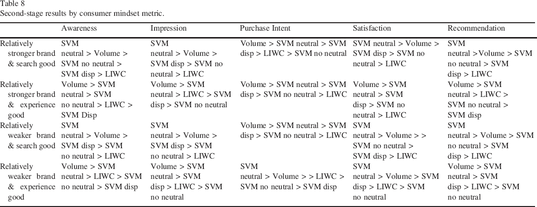
To give concrete managerial insights into these conditions, we display the rank order of the analyzed SET tools in the 20 cells of Table 8 and summarize the latter insights in a 2 × 2 in Table 9.

Table 8

Second-stage results by consumer mindset metric.

	Awareness	Impression	Purchase Intent	Satisfaction	Recommendation
Relatively stronger brand & search good	SVM neutral > Volume > SVM no neutral > SVM disp > LIWC	SVM neutral > Volume > SVM disp > SVM no neutral > LIWC	Volume > SVM neutral > SVM disp > LIWC > SVM no neutral	SVM neutral > Volume > SVM disp > SVM no neutral > LIWC	SVM neutral > Volume > SVM no neutral > SVM disp > LIWC
Relatively stronger brand & experience good	Volume > SVM neutral > SVM no neutral > LIWC > SVM Disp	Volume > SVM neutral > LIWC > SVM disp > SVM no neutral	Volume > SVM neutral > SVM disp > SVM no neutral > LIWC	Volume > SVM neutral > SVM disp > SVM no neutral > LIWC	Volume > SVM neutral > LIWC > SVM no neutral > SVM disp
Relatively weaker brand & search good	SVM neutral > Volume > SVM disp > SVM no neutral > LIWC	SVM neutral > Volume > SVM disp > SVM no neutral > LIWC	Volume > SVM neutral > SVM disp > SVM no neutral > LIWC	SVM neutral > Volume > > SVM no neutral > SVM disp > LIWC	SVM neutral > Volume > SVM no neutral > SVM disp > LIWC
Relatively weaker brand & experience good	Volume > SVM neutral > LIWC > SVM no neutral > SVM disp	Volume > SVM neutral > SVM disp > LIWC > SVM no neutral	SVM neutral > Volume > > LIWC > SVM no neutral > SVM disp	SVM neutral > Volume > SVM disp > LIWC > SVM no neutral	Volume > SVM neutral > SVM disp > LIWC > SVM no neutral

Table 9

Overview and brand examples of the contingency findings.

	Experience good	Search good
Higher brand strength	Volume suffices	Always use SVM with Neutral unless when predicting Purchase Intent (Volume)
	• Volume is the best metric• SVM neutral has second highest performance	• SVM neutral is the best metric for Awareness, Impression, Satisfaction and Recommendation• Volume is best for Purchase Intent
Example brands	• Burger King (Gastronomy)• Ford (Cars)	• Samsung (Electronics)• Southwest (Airlines)
Lower brand strength	Volume best for pre and post-purchase	Always use SVM with Neutral unless when predicting Purchase Intent (Volume)
	• Volume is the best metric for Awareness, Impression and Recommendation.• SVM Neutral is best for Purchase Intent and Satisfaction	• SVM neutral is the best metric for Awareness, Impression, Satisfaction and Recommendation• Volume is best for Purchase Intent
Example brands	• Rabobank (Banking)• Donato's (Gastronomy)	• Lenovo (Electronics)• Aeropostale (Fashion)

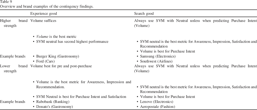
Table 8 shows the dominance of SVM Neutral and Volume SET alternatives for all attitude metrics and brand/category split-half combinations. SVM Neutral is better than Volume for search goods, with the exception of explaining Purchase Intent. For experience goods, Volume metrics typically yield the highest explanatory power, with the exception of Purchase Intent and Satisfaction for relatively weaker brands. This is consistent with a general “sentiment clarity” explanation: social media commenters use clear language when talking about recommendation and purchase intent for experience product—especially for relatively weaker brands that are less known to the public. In contrast, they can use subtle innuendos for relatively stronger brands and for search products.

Consistent with our conceptual framework in Fig. 1, but now more detailed thanks to empirical evidence, Table 9 further summarizes the results in a 2 × 2 matrix. For managers in search categories, bottom-up approaches such as SVM-with neural yield the highest explanatory power for each attitude measure apart from Purchase Intent for which they are advised to use the pre-SET volume metrics. In contrast, managers of relatively stronger brands in the experience goods category get the highest explanatory power for volume SETs. For relatively weaker brands in such category, managers should Volume to predict Awareness, Impression and Recommendation and use SVM with neutral to predict Purchase Intent and Satisfaction. Our findings thus allow brand managers in such conditions to focus on the most appropriate metrics in explaining brand attitudes.

Additional Analysis

Industry-Level Analysis: We conduct an industry-level analysis by estimating a panel vector autoregressive model by industry (for details see Web Appendix F). Volume metrics explain most of the brand awareness and impression in the banking industry, while SVM Dispersion explains all mindset metrics in the electronics industry.

Forecasting: Web Appendix G shows the out-of-sample forecasting accuracy of the five main and five combined models. The different SETs largely maintain their rank order in performance from explanation to forecasting power. The key exception occurs for the combination models, which forecast worse than the separate SET models. This is likely due to overfitting, as simpler models generally outperform complicated models in forecasting (Armstrong, 2001).

Conclusions

This paper is the first to compare how different SETs perform in explaining consumer mindset metrics. Thus, it guides marketing academic researchers and company analysts in their SET choices. We reviewed the origins and algorithms of these SETs and compared the most prominent versions for 48 unique brands in 8 industries. Using the most readily available pre-SET volume-based metrics, we collected the number of likes, comments and shares of brand posts. Next, we employed the frequently used dictionary top-down approach (LIWC) and a in the industry frequently used bottom-up approach (SVM) to extract sentiment from textual data (user comments and user posts on brand Facebook pages). Daily data for five consumer mindset metrics were combined with the differently aggregated SETs on a total of 5 million comments, which resulted in 27,956 brand-day observations for estimating VAR models and deriving the FEVD for each brand and mindset metric.

We show that there is no single method that always predicts attitudes best – a finding consistent with our expectations and the general conclusion by Ribeiro, Araújo, Gonçalves, André Gonçalves, and Benevenuto (2016) comparing among top-down approaches. On average, the most elaborate bottom-up approach of SVM Neutral has the highest R² and FEVD (dynamic R²) for brand impression, satisfaction and recommendation, while SET Volume of likes, comments, and shares has the highest R² and FEVD for awareness and purchase intent. Combining SETs yields a higher explanatory power and dynamic R².

Our findings systematically vary by mindset metrics, by brand strength, by the type of good (search vs experience good) and by industry sentiment. Volume metrics explain the most for brand awareness and Purchase Intent (Table 5) while bottom-up Support Vector Machines excel at explaining and forecasting the brand impression to satisfaction and recommendation.

When brands are both relatively stronger and part of experience goods category, they should use pre-SET volume metrics for explaining all consumer mindset metrics. For relatively weaker brands of experience goods, it is still worth using SVM with neutral comments to predict Purchase Intent and Satisfaction. In contrast, if relatively weaker brands are part of a search good category, they should invest resources for adding neutral comments to their SVM. This is particularly important for Recommendation metric. Given that product recommendations are key for search goods, relatively weaker brands can largely benefit from more complex bottom-up SETs.

Summing up, the most nuanced version of bottom-up SETs (SVM with Neutral) performs best for search goods for all consumer mind-set metrics but Purchase Intent for which Volume metrics works best. For experience goods, Volume outperforms SVM with Neutral.

How could these insights be operationalized in a company environment? First, managers should decide how precisely they want to explain and forecast customer mindset metrics. Previous studies have shown the substantial impact of these metrics on brand sales and company stock performance (e.g., Colicev et al., 2018; Srinivasan, Vanhuele, & Pauwels, 2010), but the extent to which better explanations and forecasts improve decisions is up to each company. This knowledge will help managers make cost–benefit tradeoffs among the different metrics. Volume metrics are the least expensive to obtain and perform well for explaining awareness and purchase intent. Likewise, the language dictionary of LIWC efficiently explains brand recommendation, especially for relatively stronger brands. However, both SETs are outperformed by more sophisticated machine learning techniques for explaining other metrics, especially for smaller brands. Managers of these brands should make an informed tradeoff between cost and a more nuanced understanding of sentiment in social media.

The limitations of the current study also provide avenues for future research. First, the data should be expanded to marketplace performance metrics, such as brand sales and/or financial market metrics, including abnormal stock returns (KatsikeasMorgan, Leonidou, & Hult, 2016; Hanssens & Pauwels, 2016). We expect that our results can be generalized to these ‘hard’ performance metrics because they have been quantitatively related to consumer mindset metrics in previous research (Hanssens, Pauwels, Srinivasan, Vanhuele, & Gokhan, 2014; Srinivasan, Vanhuele, & Pauwels, 2010). Second, researchers can include other social media platforms, such as blogs, microblogs and image-based platforms (e.g., Instagram). Third, newly emerging versions of our studied SETs as well as other specifications should be compared against existing options. We encourage future research to examine the suitability of more distinguished top-down approaches that rely on finer and richer dictionaries (e.g., NRC) or to focus on nuances within existing dictionaries. Likewise, though results across studies about the suitability of Random Forests and Deep Learning remain inconsistent, we encourage future research to benchmark these new and upcoming methods with the ones used in this study. Furthermore, a broader set of brands and countries would facilitate the testing of further contingencies. At a deeper level, we encourage further research to directly infer customer attitude from the underlying text, which would require either training data with a direct link between attitude and text (for bottom-up approaches), or a dictionary with synonyms of “purchase intent,” “aware,” etc. (for top-down approaches). Finally, the creation of user generated content is not equally distributed among brand-owned Facebook pages. Some brands (e.g., Audi) allow users to post on their official presence, while other brands (e.g., JP Morgan) only allow users to comment (and not post) in reply to the brand's posts. Future research might investigate how these differences in posting rights can affect the distribution of positive and negative content on brand's Facebook pages.

Social media has become an important data source for organizations to monitor how they are perceived by key constituencies. Gaining useful and consistent information for these data requires a careful selection of the appropriate sentiment extraction tool.