
Abstract
Smartphones promise great potential for personality science to study people's everyday life behaviours. Even though personality psychologists have become increasingly interested in the study of personality states, associations between smartphone data and personality states have not yet been investigated. This study provides a first step towards understanding how smartphones may be used for behavioural assessment of personality states. We explored the relationships between Big Five personality states and data from smartphone sensors and usage logs. On the basis of the existing literature, we first compiled a set of behavioural and situational indicators, which are potentially related to personality states. We then applied them on an experience sampling data set containing 5748 personality state responses that are self–assessments of 30 minutes timeframes and corresponding smartphone data. We used machine learning analyses to investigate the predictability of personality states from the set of indicators. The results showed that only for extraversion, smartphone data (specifically, ambient noise level) were informative beyond what could be predicted based on time and day of the week alone. The results point to continuing challenges in realizing the potential of smartphone data for psychological research. © 2020 The Authors. European Journal of Personality published by John Wiley & Sons Ltd on behalf of European Association of Personality Psychology
Introduction
With mobile sensing methods, personality science is gaining new opportunities for studying people's behaviours in daily life (Harari et al., 2016; Stachl et al., 2020a). As an innovative approach for unobtrusive ambulatory behavioural assessments (Trull & Ebner–Priemer, 2014), mobile sensing using everyday devices that many people carry around most of their day (e.g. smartphones) is particularly promising, as data from these devices can readily be collected and potentially reflects many daily life behaviours and situations.
Indeed, smartphones have not only been touted as potentially transformational for psychology research (Harari et al., 2016; Harari, Müller, Aung, & Rentfrow, 2017; Miller, 2012), but they have also already been applied in personality science to examine associations with personality traits. Extant research indicates that personality traits are associated with a variety of behaviours that can be, at least partially, measured by smartphones. Examples are making phone calls (Montag et al., 2014), following a regular daily routine (Wang et al., 2018), and spending time in the company of others, as recorded through the detection of nearby Bluetooth devices (Harari, Gosling, Wang, & Campbell, 2015; Wang & Marsella, 2017).
However, relations between smartphone data (defined as data from smartphone sensors and smartphone usage logs) and personality states have so far not been explored. Personality states describe how traits are expressed or manifested in daily life situations (Baumert et al., 2017; Fleeson, 2001; Horstmann & Ziegler, 2020) and have recently received increasing attention in personality research, due to the need for integrating trait and process approaches (Finnigan & Vazire, 2018; Fleeson, 2017; Geukes, Nestler, Hutteman, Küfner, & Back, 2017; Horstmann & Ziegler, 2020; Sened, Lazarus, Gleason, Rafaeli, & Fleeson, 2018; Sherman, Rauthmann, Brown, Serfass, & Jones, 2015; Wrzus & Mehl, 2015). Understanding how smartphone data relate to personality states may constitute a first step towards behavioural assessment of personality states, because behaviours that are captured by smartphone data and are associated with a personality state may be part of the state's behavioural manifestations. Furthermore, situation characteristics that are captured by smartphone data may also contribute towards unobtrusive assessment of personality states, as they potentially constitute situational determinants of the personality state.
In general, inferences about behaviours and situations based on smartphone data may be relevant both as a complement and (partial) substitute to survey assessments when studying or assessing expressions of personality in daily life. More concretely, it could benefit the following applications. First, as development and validation of survey measures of personality states is currently an active area of research (Horstmann & Ziegler, 2020), smartphone data may be useful for both assessing their external validity (by revealing association with conceptually related behaviours and situations) as well as reliability (by revealing reliable contingencies between states and situations, see Horstmann & Ziegler, 2020). Second, smartphone data may be useful for developing, testing, and refining theories that involve personality states, such as whole trait theory (Fleeson & Jayawickreme, 2015). Third, it may be relevant for testing the effectiveness of interventions that are designed to affect personality traits (such as Magidson, Roberts, Collado–Rodriguez, & Lejuez, 2014; Stieger et al., 2020), because the corresponding state measures should be affected by changes in the trait variable (Horstmann & Ziegler, 2020). Finally, it may allow reducing the burden of survey assessment for study participants by triggering the surveys only when change of behavioural patterns suggest a change in personality state patterns.
The present study investigates the associations between smartphone data and self–assessed Big Five personality states (referring to the past 30 minutes), as a first step towards the application of smartphone data in the context of personality states. To match the context of the self–assessment, we used the smartphone data collected during the same 30 minutes. We chose this timeframe to ensure a minimal amount of sensor data, to capture relatively short–term variation of personality states, and to allow comparison with related work (Kalimeri, Lepri, & Pianesi, 2013).
Before introducing our study, we discuss three topics of previous research. First, as this study and much of the existing literature are based on exploratory analysis using machine learning techniques (Breiman, 2001b; Yarkoni & Westfall, 2017), we first highlight the relevant characteristics of this application of machine learning. As personality states and traits are closely related, and due to the existing literature's focus on traits, we then briefly summarize relevant existing work with respect to personality traits. Finally, we describe available research on personality states.
Exploratory analysis using machine learning
A number of articles have highlighted the potential of machine learning approaches for personality research (Bleidorn & Hopwood, 2018; Stachl et al., 2020a; Yarkoni & Westfall, 2017). They emphasized a number of strengths, including the ability to handle a large number of predictor variables even with relatively small data sets, and the potential to achieve high prediction performance (Yarkoni & Westfall, 2017). In the current work, we focus on the application of machine learning for exploratory analysis, which is a common use of machine learning in various research fields (e.g. Inza et al., 2010; Oquendo et al., 2012; Wu et al., 2016) but has, to the best of our knowledge, so far received little explicit attention in psychology (for rare examples, see Adjerid & Kelley, 2018; Aichele, Rabbitt, & Ghisletta, 2016; Aschwanden et al., 2020). Nevertheless, it has previously been applied in personality studies (e.g. Mønsted, Mollgaard, & Mathiesen, 2018; Stachl et al., 2020b; Stieger et al., 2020). Like in these studies, exploratory analysis using machine learning often consists of creating predictive models using a variety of predictor variables and either evaluating the contribution of individual variables or sets of variables, or selecting a subset of relevant predictor variables. This approach, which we also apply, can elucidate limits of predictability as well as reveal interesting and understandable associations between the predictor variables and the predicted target variable. This is possible despite the fact that machine learning models are often seen as ‘black boxes’, which may give accurate predictions, and yet are too complex to be meaningfully understood and interpreted (Yarkoni & Westfall, 2017). The reason is twofold. First, there is a trade–off between interpretability and the accuracy of prediction, and there exist machine learning techniques that offer a balance of both (James, Witten, Hastie, & Tibshirani, 2013). Second, the machine learning research community has been actively developing new methods for model interpretation (Du, Liu, & Hu, 2019; Guidotti et al., 2018). In most cases, it is therefore possible to achieve at least some degree of interpretability. Furthermore, even a black box model that simply shows that a target variable is predictable from a set of inputs can be an informative result, if this outcome was unexpected (Holm, 2019). It should be noted that while this approach is suited for exploring a larger set of predictors compared with traditional approaches, including additional irrelevant predictors will nevertheless tend to lead to less accurate assessment of the relevance of each predictor, as well as an underestimation of predictive performance. Therefore, the predictors should still be carefully selected.
In summary, machine learning approaches are useful for exploring predictability and revealing associations between predictor variables and the target variable when the number of predictor variables is large. In the following subsection, we discuss literature that has linked smartphone data and personality traits, often based on exploratory analysis using machine learning.
Smartphone data and personality traits
At least two research streams relate to the associations between personality traits and smartphone data. The first growing research stream has focused on the predictability of self–reported Big Five personality traits from smartphone data (e.g. Chittaranjan, Blom, & Gatica–Perez, 2011; De Montjoye, Quoidbach, Robic, & Pentland, 2013; Mønsted et al., 2018; Stachl et al., 2020b; Wang & Marsella, 2017; Wang et al., 2018; Xu, Frey, Fleisch, & Ilic, 2016). Previous research on the predictability of traits proposed and evaluated a broad range of behavioural indicators for inference of personality traits and demonstrated that personality traits could be predicted above the level of chance using machine learning techniques (e.g. Chittaranjan et al., 2011). The most extensive analysis to date investigated the predictability of Big Five traits using smartphone data from 624 participants and a set of 1821 indicators (Stachl et al., 2020b). On the trait level, they found the highest predictability for extraversion, and no predictability for agreeableness. Indicators important for prediction of extraversion were mostly related to communication and social behaviour (based on call, message, and communication app–usage logs); for openness, it was app–usage, and communication and social behaviour. Conscientiousness was related to indicators of daily routine and app–usage. Only some facets of emotional stability could be predicted, mostly relying on indicators from communication and social behaviour, unlock frequency, and app–usage.
Within this research stream, only one study investigated whether previous findings generalize to an independent and larger data set from 636 study participants (Mønsted et al., 2018). In this study, only extraversion could be predicted above the level of chance. This may be due to the rather small set of 22 predictors that were mainly related to communication (calling and texting). Furthermore, the authors argued that the predictability reported in the study by De Montjoye et al. (2013) may have been overestimated due to methodological limitations.
A second, more diverse literature stream did not explicitly focus on the prediction of personality from smartphone data but nevertheless reported associations between smartphone data and personality traits (Harari et al., 2019; Montag et al., 2014; Montag et al., 2015; Schoedel et al., 2020; Servia–Rodriguez et al., 2017; Stachl et al., 2017). One of the earliest large studies investigated usage patterns of WhatsApp and other mobile applications and found that extraversion was positively associated with the duration of daily WhatsApp use, while conscientiousness was negatively related (Montag et al., 2015). A recent study focused on sensing of sociability using smartphones and found, as expected, the strongest associations with extraversion, compared with the other Big Five traits (Harari et al., 2019). Fewer and weaker associations were found for openness and neuroticism, while very few associations were found for agreeableness and conscientiousness. Another study examined day–night behaviour patterns in smartphone data and found associations with conscientiousness and extraversion (Schoedel et al., 2020). Furthermore, mobile sensing research investigated social interactions, daily activities, and mobility patterns that might be related to personality traits (Harari et al., 2016). For instance, an analysis of location–based social network data evidenced associations between mobility patterns and both neuroticism and openness.
Taken together, of all Big Five personality traits, extraversion has been linked to smartphone data most consistently. In the following subsection, we will briefly discuss the two only studies so far that have assessed the momentary fluctuations in personality states by mobile sensing methods, albeit not with smartphones.
Smartphone data and personality states
Personality traits and personality states are conceptualized as having the same content (i.e. behaviour, cognition, and affect; Baumert et al., 2017) albeit with different time frames (in general vs. momentary) and a difference in context–dependence. Personality traits explicitly disregard context, referring to characteristics ‘in general’, whereas personality states are understood to depend on the situational context. Essentially, personality states are characteristics of individuals that change over short–term time periods and vary across specific situations. So far, to the best of our knowledge, no studies have investigated associations between personality states and smartphone data. Nonetheless, at least two studies investigated links between data from a specialized mobile device (i.e. the sociometric badge, which is worn on the chest, Olguin et al., 2009) and personality states, assessed on the past 30 minutes (Kalimeri et al., 2013; Teso, Staiano, Lepri, Passerini, & Pianesi, 2013). The first study found that data from each of the badge's sensors individually were predictive of the personality state for each Big Five dimension, and a combination of data from different sensors yielded higher predictability (Kalimeri et al., 2013). The second study found that indicators based on graph structure representations of social interaction patterns also predicted states of all Big Five dimensions (Teso et al., 2013). Smartphones have both important commonalities and differences with sociometric badges. First, they are similar enough for suggesting associations between smartphone data and personality states. As they share two sensors, Bluetooth and microphone, results from the sociometric badges may partly generalize to smartphones. However, they are different enough that we cannot expect to find the same associations as with personality states. They differ in important ways such as energy resources available for unobtrusive data collection and the interaction between the device and the study participant. Furthermore, these differences imply that, while the studies with sociometric badges allowed to passively collect high–resolution longitudinal data due to the specialized device, they were limited to the work environment of the participants. Furthermore, the sample that could be investigated was likely limited by issues of device cost, user adoption, and distribution. Even though smartphones offer a broader variety of behavioural data sources, are habitually carried around by their users for most of their day, and are accessible to almost everyone (Poushter, 2016), they have so far not been used in the context of studying personality states.
Similar to the trait literature, research on the link between situational cues and personality states may inform the extraction of useful smartphone indicators. For example, situational cues, such as location (i.e. whether a person is at home, at work or at another significant location; Montoliu, Blom, & Gatica–Perez, 2013) and social cues (e.g. the presence of specific other people; Chen et al., 2014) are inferable from smartphone data and likely linked to personality states (Harari et al., 2015). For example, people may be more disciplined at work than at home and when others are present (Hofmann, Baumeister, Förster, & Vohs, 2012). Thus, conscientiousness may be associated with both significant locations and presence of others. Similarly, the workplace is often a source of stress (Lazarus, 1995), which can trigger anxiety and negative affect, whereas friends and family members are often providers of emotional support (Cohen, Sherrod, & Clark, 1986), and thus, both likely impact state neuroticism. Finally, sociability is conceptually a part of extraversion (John, Naumann, & Soto, 2008) and also related to the presence of others.
In summary, there exists literature that suggests associations between personality states and smartphone data, but so far, these have not been examined. In the following section, we will therefore outline how our study addresses this research gap.
The current work
To the best of our knowledge, this study is the first to investigate associations between Big Five personality states and smartphone data. Focusing on the within–person dynamics, our research therefore explored associations between ipsatized self–reported personality states referring to the previous 30 minutes, and smartphone data captured during the same 30 minutes. Ipsatization refers to the procedure of subtracting every participant's mean state value from their reported state values (He et al., 2017). As a prerequisite to the analysis, we developed and computed indicators of behaviours and situations that may be linked to personality states. Three rounds of analyses were conducted to explore the associations between the indicators and personality states. In a first step, pairwise correlations between indicators and personality states were explored. In a second step, machine learning methods were used to analyse the predictability of personality states from the indicators. In a third step, feature selection was used to determine the subset of indicators that were relevant for prediction. In the following section, we outline each of these steps of the analysis in detail.
Method
Data set
Data come from an intervention study (Stieger et al., 2018), whose purpose was to test the effectiveness of a smartphone–based 10–week digital coaching intervention for intentional personality change. We restricted our analysis to the experience sampling data that were collected in the first week of the study without any intervention components. While we cannot make the raw smartphone data public due to privacy issues, the computed indicator values along with the survey responses and scripts are available at https://osf.io/j93bs/.
Participants
The initial sample consisted of 1523 adults who downloaded and installed the PEACH app (Android or iOS version) on their smartphone and participated in the initial assessment. Participants were recruited via mailing lists and advertisements on social media. For the present analysis, we only examined data from participants who used an Android device (47%) and provided at least one experience sampling response. Users of iOS devices (53%) were excluded, because the iOS platform prevents apps from accessing relevant data like the full list of nearby Bluetooth devices, and, as also noted by Harari et al. (2019), the phone call log. We also excluded 35 participants for whom the smartphone data were missing, presumably because they uninstalled the app before the data could be uploaded. Furthermore, we excluded 93 participants that completed less than 10 personality state surveys each, in order to ensure sufficient accuracy for participant–wise centring of the state variables. This resulted in a final sample of 316 participants (51% male) with an average age of 25.1 years (SD = 7.0 years). From the participants, 54% were students, 26% were in full–time employment, and 18% were in part–time employment.
Procedure
In the first week of the intervention study, participants completed an experience sampling phase of 6 days (Monday to Saturday), during which surveys were triggered four times per day at random times in predefined time windows (9:30 a.m. to 11:30 a.m., 12:30 p.m. to 2:30 p.m., 3:30 p.m. to 5:30 p.m., and 6:30 p.m. to 8:30 p.m.) to complete short self–reports. While the selected participants provided a total of 5748 experience sampling responses (out of a total of 7584 measurement occasions, 316 participants × 4 assessments per day × 6 days), the PEACH mobile application collected sensor data and usage logs, which resulted in a final set of 5748 responses with corresponding smartphone data for our analysis.
Self–report measures
The experience sampling included an assessment of Big Five personality states in the last 30 minutes using 10 bipolar adjective item pairs on a slider scale ranging from 0 to 100 (two per personality trait, presentation in a random order, similar to Geukes et al., 2017; Schmukle, Back, & Egloff, 2008). The items were ‘close–minded–open–minded’ and ‘uninterested–curious’ for openness, ‘imprudent–deliberate’ and ‘unconscientious–conscientious’ for conscientiousness, ‘quiet–talkative’ and ‘shy–outgoing’ for extraversion, ‘insensitive–empathic’ and ‘distrustful–trusting’ for agreeableness, and ‘tense–relaxed’ and ‘unconfident–self–confident’ for neuroticism. Please see Appendix A for the original German versions of the adjectives that were used in the study, the histograms of the measurements, and an illustration of the user interface. The descriptive statistics of the measurements are given in Table 1.
Descriptive statistics of 5748 available state measurements (scale: 0 to 100)
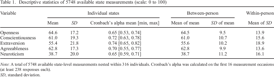
Note: A total of 5748 available state–level measurements nested within 316 individuals. Cronbach's alpha was calculated on the first 16 measurement occasions (at least 238 responses each).
SD, standard deviation.
It is notable that the distribution of the extraversion measure appears somewhat different from the other measures. It is wider, with the mean closer to the centre of the scale, and with a somewhat bimodal shape due to a relatively low number of responses around the mean of the distribution. The wider shape reflects the larger within–person variability, which is only partially consistent with related work, where the largest within–person variabilities were found for both conscientiousness and extraversion (Bleidorn, 2009; Fleeson, 2007).
In all further analyses, we used ipsatized state responses, that is, we centred the responses for each participant and measure, which in principle removes between–person variability by controlling for participant–level factors that influence the responses.
Unobtrusive smartphone data collection
The study app used the open source MobileCoach platform for behavioural interventions and ecological momentary assessments (Kowatsch et al., 2017) and included a module for recording sensor data and usage logs derived from the EmotionSense open source library (Lathia, Rachuri, Mascolo, & Roussos, 2013). Based on the available literature, we decided to record data from the sensors and usage logs as outlined in Table 2 and with the following considerations: first, previous work had linked sensor and usage log data to specific personality traits both directly (Chittaranjan et al., 2011; De Montjoye et al., 2013; Rüegger, Stieger, Flückiger, Allemand, & Kowatsch, 2017; Servia–Rodriguez et al., 2017) and indirectly through categories of behaviour (Chorley, Whitaker, & Allen, 2015; Harari et al., 2016; Hirsh, DeYoung, & Peterson, 2009). These associations potentially also exist for corresponding states, due to the equality of their content (i.e. they describe the same behaviours, cognitions, and affects). Second, even though smartphones and the sociometric badge differ in important ways, they share two sensors, Bluetooth and microphone, which have been shown to be related to personality states (Kalimeri et al., 2013). Finally, smartphone data may be linked to personality states through situational cues (Chen et al., 2014; Cohen et al., 1986; Harari et al., 2015; John et al., 2008; Lazarus, 1995; Montoliu et al., 2013).
Sensor and usage log data collection
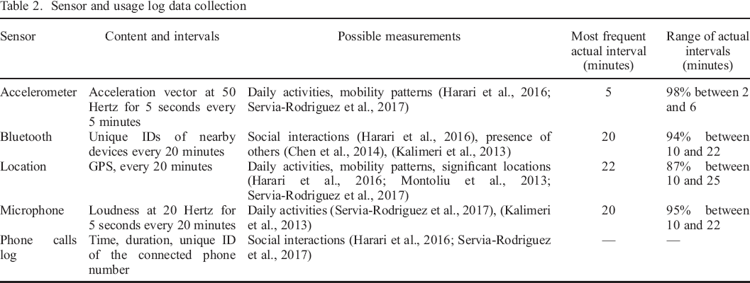
The contents and sampling intervals of the data collection are listed in Table 2. For exploratory purposes, we also recorded additional samples at shorter intervals (i.e. half of the main interval, typically 10 minutes) at random time points. Therefore, Table 2 also lists the actually observed intervals (see the last two columns).
The relatively large sampling intervals (up to about 20 minutes) and, for accelerometer and microphone data, short sampling durations (5 seconds), were chosen to allow recording at the same rates over a full day without impacting battery life too much. Nevertheless, a large fraction (29%) of people who had dropped out of the study indicated battery drain as a reason for no longer participating. Such a sampling scheme can be understood as adding considerable noise to the data, because what is observed at distinct and interspaced points in time may not be representative of a longer time period. Within the current work, because of this limitation in the data collection, we can therefore expect to find only the strongest of the associations that exist between personality states and smartphone data.
While data collection generally happened in the background without requiring effort from the study participants, for Bluetooth and location sensing, we depended on participants to keep Bluetooth connectivity and background geolocation enabled on their phone. Therefore, if any of these functionalities was disabled, the app asked the participant at most every 48 hours to enable it.
Developing behavioural and situational indicators
We created a list of behavioural and situational indicators that are potentially associated with personality states based on reported associations with both traits and states in prior work (Adalı & Golbeck, 2014; Chittaranjan et al., 2011; De Montjoye et al., 2013; Grover & Mark, 2017; Kalimeri et al., 2013; Mønsted et al., 2018; Servia–Rodriguez et al., 2017; Stachl et al., 2020; H. Wang & Marsella, 2017). We considered only the indicators that we could use based on the collected data set. Some indicators are partly based on data collected during the whole baseline week, which can serve to identify, for example, home and work locations, and Bluetooth devices that were co–located in multiple places.
In the following paragraphs, we discuss each method that we applied to derive the indicators.
Adapting trait indicators
The proposed indicators from the existing literature on prediction of personality traits can be assigned to one of two classes: indicators of the quantity of behaviours and indicators of the variability of behaviours. Quantity–based indicators relate to the frequency or duration of behaviours. Examples are the number of outgoing phone calls and the sum of their durations. Variability–based indicators refer to, for example, the variance of the time between calls or the extent to which smartphone use follows a 24–hour rhythm. For our analysis, we used indicators that (1) have been observed as associated with Big Five personality traits and (2) represent a sum, maximum or average level of a quantity which is related to a behaviour. An example is the total duration of phone calls, which was associated with trait extraversion (Chittaranjan et al., 2011). In this case, we can expect that the behaviour is potentially also associated with the corresponding personality state (i.e. talking on the phone may be associated with state extraversion), as experience sampling studies have found that a higher average level of a self–reported personality state was associated with a higher level of the corresponding trait (Fleeson & Gallagher, 2009). Note that it is not always possible to classify indicators strictly into either ‘behavioural’ or ‘situational’. For example, indicators based on loudness of sound recorded by the microphone capture sounds generated through behaviour (e.g. talking and moving), as well as the environment. Furthermore, the act of staying in a particular environment can be strongly related to certain behaviours or can even be considered a behaviour in itself. Therefore, in order to explore a broader range of indicators, we included these cases as well. As for the process of adapting the trait indicators for states, it is simple: because they represent a sum, maximum or average level observed within a certain time frame, we can simply compute them over a shorter time frame. For the list of derived indicators, the names of the corresponding trait indicators and their reported associations with Big Five traits, see Table 3. We determined the associations for the indicators from Stachl et al. (2020) based on their published data, as described in Appendix B. We included indicators from studies with relatively small samples based on the reasoning that we are seeking to explore a broad range of indicators and that even these studies provide at least some evidence for associations that are relevant for personality states.
List of indicators and reported associations with Big Five
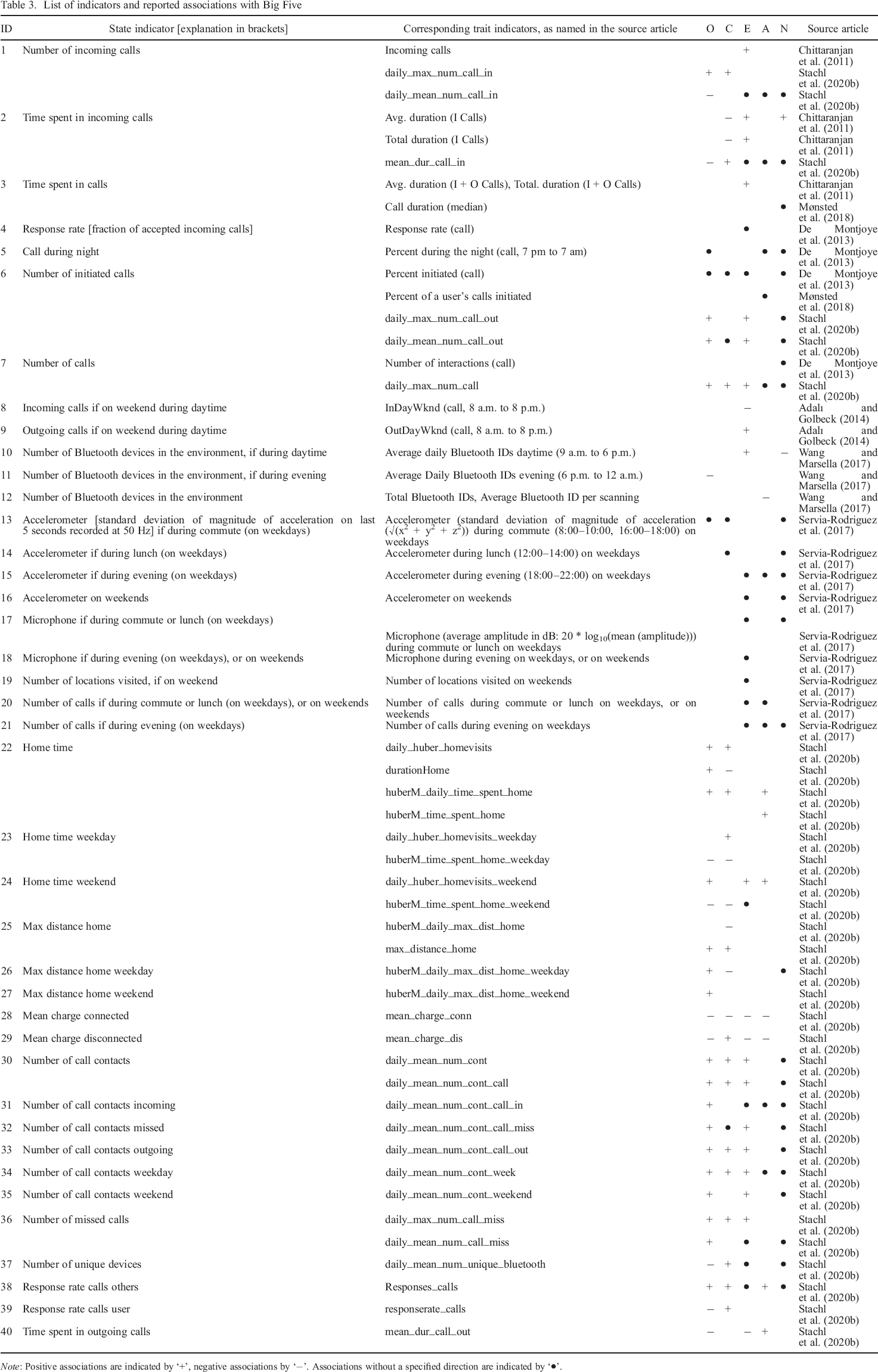
Note: Positive associations are indicated by ‘+’, negative associations by ‘−’. Associations without a specified direction are indicated by ‘•’.
Adapting state indicators from the sociometric badge
Studies that related data from the sociometric badge to personality states can also serve as a source of indicators for this work, because smartphones share two sensors with the sociometric badge (i.e. Bluetooth and microphone). On the basis of the relevant literature on assessing Big Five states (Kalimeri et al., 2013), we use the indicators outlined in Table 4. Some of their indicators could not be used, because they are based on survey data about the participant's relationships with the wearers of the detected Bluetooth devices, which is not available in the present study. Other indicators needed to be adapted: in Kalimeri et al. (2013), indicators such as ‘mean amplitude’ and ‘standard deviation’ of the audio data were only computed on the part of the signal that was classified as ‘speaking’. However, we did not apply speaking detection in the present study for reasons of battery efficiency. With the expectation that at least some of the meaning of the indicators may be preserved, we therefore applied the microphone indicators on all microphone samples. Also, we adapted the indicators that provide a distance measure of nearby devices based on the strength of Bluetooth signals (for details, see Appendix C). Note that, again, these indicators cannot be strictly separated into either situational or behavioural types.
Indicators from sociometric badge studies and reported associations with Big Five

Note: The symbol ‘•’ indicates associations without a specified direction.
RSSI, Received Signal Strength Indicator.
Additional situational indicators
We propose additional indicators, which have not previously been used in the context of studying Big Five personality with mobile devices and which can arguably be seen as primarily situational. The indicators belong to two categories. The first category is based on classification of locations: we use the approximate fraction of time within the time frame that is spent at locations of different classes (work, home, ‘home office’, or other). This is motivated by research that relates location cues to personality states (Cooper & Marshall, 1976; Hofmann et al., 2012). For a description of how we assigned the classes, see Appendix C. The second category is based on classification of Bluetooth devices. We use the number of sensed nearby devices, counted for each class. Nearby devices sensed via Bluetooth may indicate the presence of a colleague, friend, or romantic partner. However, from the Bluetooth sensor, we do not receive the information about whether a device is a personal device of another person (rather than one belonging to the participant, e.g. a smartwatch), or what the relationship with that person is. Nevertheless, in an attempt to approximate this information, we classify devices based on the classes of locations at which they have been observed. The underlying rationale is that a device observed at home and other locations may indicate a romantic partner, family member, or cohabitant, who is likely a provider of emotional support and thus may influence state neuroticism. Likewise, a device observed at work and other locations may indicate a co–worker who is also a friend. However, a device observed at all three types of locations may more likely belong to the participant, for example a laptop or smartwatch. On the basis of these considerations, we propose the indicators and potential associations as outlined in Table 5.
Proposed situational indicators and potential associations
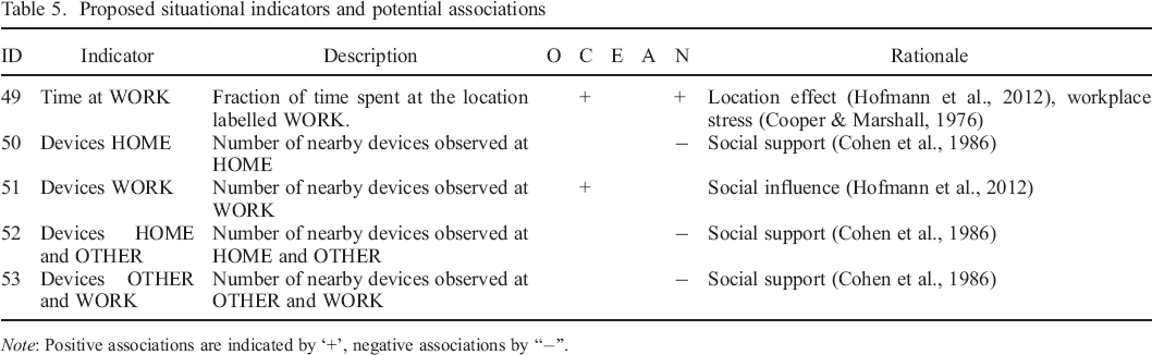
Note: Positive associations are indicated by ‘+’, negative associations by “−”.
Generalized indicators
Some indicators that we adapted from previous research are combinations of situations and behaviour, for example, the number of calls during the night or the number of incoming calls during the weekend. This leads to some indicators that are very sparse, that is, many values are zero or missing. Thus, there may be too little variability in these indicators to detect any associations with personality states. Therefore, we exploratively added more general versions of these indicators that do not take any context into account (Table 6).
Generalized indicators
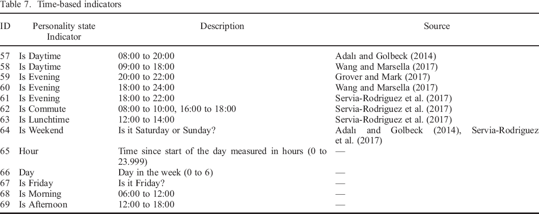
Time–based indicators
Time is a situational component (Rauthmann, Sherman, & Funder, 2015), which has been shown to be associated with personality states (Fleeson, 2001), in line with ample evidence for diurnal patterns of behaviour and affect (Golder & Macy, 2011; Harari et al., 2019; Servia–Rodriguez et al., 2017). However, time has not yet been considered in the context of research that examines associations between mobile sensing data and personality states (Kalimeri et al., 2013; Teso et al., 2013). Not considering time as a situational indicator can lead to irrelevant indicators showing associations with personality states, simply because they also follow daily or weekly cycles. Essentially, we use time–based indicators as control variables and as a baseline for assessing the potential of smartphone data for state assessment. From a state assessment point of view, finding that smartphone data cannot tell us more about personality states than what can be predicted by time alone suggests that it is irrelevant. We used time–based indicators that are based on trait–level indicators from previous work (Adalı & Golbeck, 2014; Grover & Mark, 2017; Servia–Rodriguez et al., 2017; Wang & Marsella, 2017) and added further time–based indicator that capture complementary and potentially relevant aspects of time (Table 7). For example, we added the variable ‘Is Daytime’ and ‘Is Weekend’ based on, among others, the indicator ‘Incoming calls if on weekend during daytime’, and added ‘Is Morning’ because the concept of ‘morning’ was not used in the reviewed studies but seemed unjustifiably absent considering the presence of ‘Is Evening’ and ‘Is Lunchtime’.
Time–based indicators
Descriptive statistics of the indicators for personality states
To explore the associations between smartphone data and personality states, we focused on the smartphone data collected in the 30–minute timeframe preceding each completed experience sampling survey. Timeframes were chosen to end when the participant provided the response to the first element of the experience sampling process (photographic affect meter; Pollak, Adams, & Gay, 2011). This was done for the following two reasons. First, the self–assessment procedure asked the participants to describe their perception of the previous 30 minutes, which we approximately matched, as 95% of the intervals between the end of the timeframe and the submission of the personality state responses were shorter than 5 minutes (median: 1.5 minutes). Second, assessment itself influences behaviour and may thus influence the smartphone data that are collected during and after self–assessment, so it makes sense to include only data from before the beginning of self–assessment. For each timeframe, we calculated the set of indicators that we described in the previous subsection. The distributions of the indicators are described in Appendix D.
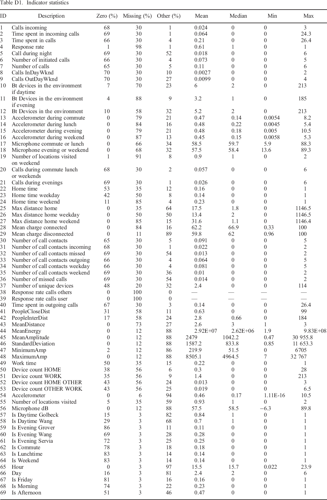
Note that many values are either missing or zero. For example, only a small number of timeframes contain at least one phone call, due to phone calls being relatively rare events. In contrast, accelerometer and microphone information are available for 96% and 89% of the timeframes, respectively. But less than half have associated information about Bluetooth devices in the environment, as many study participants did not keep Bluetooth activated on their phone, despite being asked to do so. The availability of information about location is better, at 65%. Nearly all of the distributions are heavily skewed, with many smaller values and few large ones. Note that for further analysis, we excluded two indicators because all values were missing (ID–38 and ID–39).
Data analysis
As it is challenging to make justified assumptions about the statistical form of associations between smartphone data indicators and self–assessed personality state levels, we chose an exploratory approach. In order to focus on the within–person variability, we first ipsatized the state measures. That is, we subtracted each participant's average state level from their individual/momentary state measurements for each Big Five dimension. Our analysis of the associations between ipsatized state measures and smartphone data indicators then proceeded in three steps. In a first step, we examined simple pairwise correlations between smartphone data and personality states. In a second step, we fitted and evaluated different models, focusing on machine learning models that can predict the self–assessed personality state with high accuracy. To account for the existence of more complex associations, this included models that can capture interactions between indicators. In a third step, we focused on individual indicators and their associations with personality states, by identifying subsets of indicators that are likely predictors of personality states.
Step 1—Correlation analysis
Correlations are arguably the simplest associations that may exist between personality states and smartphone data. We therefore examined the pairwise correlations between each indicator and each state measure. In line with related work (Mønsted et al., 2018; Pratap et al., 2018), we also examined correlations among indicators and among state measurements, as this can be helpful for understanding the data and interpreting other results. We used Spearman's rank correlation, as the distributions of most indicators are highly skewed and non–normal.
Step 2—Prediction analysis
In this step, we focused on estimating the predictability of state measures from smartphone data. In particular, we were interested in whether smartphone data improves prediction performance beyond two baseline measures. As a first baseline, we used an approach that is independent of any indicators and instead learns the mean personality state level. For a second baseline, we used only time–based indicators. To compute these indicators, nothing more than the local time and date of the state assessment needs to be known. For state assessment applications, time and date of assessment are likely to be available independent of the data collection method.
We applied machine learning techniques, because they are suitable for prediction tasks (Yarkoni & Westfall, 2017) and because they require less a priori assumptions compared with more traditional statistical methods (Breiman, 2001b). Any machine learning analysis typically includes exploring a set of different models or approaches and then performing model selection, that is, selecting the best model or approach for the task at hand. Correctly combining estimation of predictive performance with model selection is not trivial (Tsamardinos, Rakhshani, & Lagani, 2015). The core problem is that when selecting the best performing model based on an unbiased measure that includes random measurement errors, the ‘winning’ model's performance will likely have been positively affected by chance. That is, the performance measure of this model is no longer unbiased, especially if the number of candidate models is large. In order to arrive at an unbiased estimate of the prediction performance despite this problem and following Stachl et al. (2020), we applied nested cross–validation (Varma & Simon, 2006; Yarkoni & Westfall, 2017). Cross–validation (Kohavi, 1995; Stone, 1974) is the procedure of repeatedly splitting the data into separate parts for fitting (e.g. 80% of the data) and evaluating (e.g. 20%) a prediction model, which enables the use of the entire data set for evaluation, whereas the typical alternative approach only uses a limited sample that is based on a single split and thus may be less representative of out–of–sample data. Nested cross–validation in turn refers to the use of a further, ‘nested’ cross–validation procedure as part of each model fitting process, in order to optimize any modelling choices that are not learned by the learning algorithm itself. For example, the least squares algorithm determines the coefficients of a linear model, but it does not learn which indicators should be included in the model. Instead, the choice of which indicators to include can be optimized using the nested cross–validation procedure. Note that a consequence of using nested cross–validation is that different modelling procedures can be best on different cross–validation folds. Thus, nested cross–validation may not determine a single ‘best’ model, but up to k best models in k–fold cross–validation.
To ensure that models generalize to out–of–sample participants, and in line with previous work (Chittaranjan et al., 2011; Kalimeri et al., 2013), we used participant–wise splitting (Saeb, Lonini, Jayaraman, Mohr, & Kording, 2017). Participant–wise splitting means that data from one participant are never present in both the portion of the data used for model fitting and the portion used for evaluation. For further details regarding our implementation of nested cross–validation, see Appendix E.
The first dimension identifies the learning algorithm. We explored several algorithms that are widely used for prediction problems. The first algorithm is XGBoost (Chen & Guestrin, 2016). It is an implementation of the boosted decision trees algorithm (Friedman, 2001), which has recently become a popular choice in commercial and academic machine learning competitions (Chen & Guestrin, 2016), where the goal is to achieve the highest prediction performance. It has been found on par or superior to established algorithms such as Random Forests (Breiman, 2001a) and neural networks in a diverse set of applications (Fan et al., 2018; Gupta, Shrivastava, Khosravi, & Panigrahi, 2016; Sheridan, Wang, Liaw, Ma, & Gifford, 2016). Being based on decision trees, this algorithm is both well–suited (1) to model non–linear associations, which often occur between personality and behavioural measures (Benson & Campbell, 2007; Cucina & Vasilopoulos, 2005) and (2) to model complex interaction structures (Friedman, Hastie, & Tibshirani, 2001), which can lead to high predictability despite there being only small correlations between the indicators and the target variable. A further advantage of XGBoost compared with neural networks is that it can handle missing values appropriately without the need for imputation. The second and third model are ridge regression (Hoerl & Kennard, 1970; James et al., 2013) and lasso regression (James et al., 2013; Tibshirani, 1996), which are two variations of regularized regression algorithms (Xing, Jordan, & Karp, 2001) and which have been widely used, including in personality research (Hall & Matz, 2020; Seeboth & Mõttus, 2018; Stachl et al., 2017; Stachl et al., 2019). Finally, we also explored ordinary least squares regression.
The second dimension that we explored for model selection, consists of different indicator subsets. Although machine learning can be applied even with a large number of indicators (e.g. Stachl et al., 2020), preselecting an appropriate subset of indicators for model fitting often improves the achieved prediction performance (Guyon & Elisseeff, 2003). Therefore, using only indicators that can be expected to have some association with the predicted state measure may improve the predictive performance. We thus explored two different subsets of indicators. The first set, which we will refer to as ‘Set A’, consists of only the indicators that we can expect to be potentially associated with the target state measure, based on the associations that are listed in Table 3 and following. The contents of Set A are thus specific to each Big Five dimension. The second set (‘Set B’) consists of the union of all dimension–specific versions of Set A. In other words, it includes the indicators that are potentially associated with state measures of any Big Five dimension. Set B is identical in all analyses.
The third dimension concerns the application of algorithms for addressing the challenges that are due to using a relatively large number of indicators, including with collinearities. There are several algorithms that can be applied. Indicator selection (called feature selection in machine learning terminology) consists of automatically selecting the subset of indicators that leads to the highest predictive performance. Various techniques for feature selection exist. For an optimal selection of indicators, an exhaustive search of all options would be necessary. However, this is often not feasible due to the large number of possible subsets of indicators. Like Kalimeri et al. (2013), we applied a more efficient approach, which starts with an empty set of indicators and repeatedly adds or removes individual indicators so that prediction accuracy is improved in each step. This procedure is called sequential forward floating selection (SFFS) (Pudil, Novovičová, & Kittler, 1994) and is considered to be more effective compared with alternatives (Jain & Zongker, 1997). Although SFFS can still be computationally too expensive for large sets of indicators, it is widely used (Al–Zubaidi, Mertins, Heldmann, Jauch–Chara, & Münte, 2019; Batliner et al., 2011; Pohjalainen, Räsänen, & Kadioglu, 2015), and we found it feasible to apply in our case. Only when exploring larger subsets of 16 or more indicators, we used a more efficient variant called sequential floating selection. This algorithm never removes previously added indicators, which can dramatically reduce the computational effort by reducing the number subsets that are explored, while not necessarily leading to worse solutions (Reunanen, 2003).
An alternative procedure to feature selection is principal components analysis (PCA) (Abdi & Williams, 2010), which is similar to factor analysis and consists of reducing the data to the principal dimensions along which it varies (Li & Jain, 1998), thus replacing a given set of indicators by a smaller set of derived indicators. Finally, regularization, which is used in Ridge and Lasso regression and biases coefficients towards smaller values, also addresses the problems caused by using a large number of predictors (Yarkoni & Westfall, 2017).
The final dimension that we optimized consists of the parameters that are used by the previously described techniques. Feature selection requires the specification of the number of indicators to select, and PCA requires indicating the number of principal dimensions to retain. Finally, Lasso and Ridge regression require a parameter called alpha, which determines the degree of regularization.
Step 3—Analysis of multivariate associations
Using an automated procedure for selecting relevant indicators, which we applied to increase the prediction performance of our models, also reveals the indicators that are most informative about personality states. We therefore examined results of this selection, similar to previous work by Kalimeri et al. (2013) and Mønsted et al. (2018). However, we went beyond their reporting of a single set of selected indicators, because feature selection has been recognized to be often unstable, that is, sensitive to small variations in the input (Guyon & Elisseeff, 2003). Therefore, and as suggested by Guyon and Elisseeff (2003), we counted how often a feature was selected across different subsamples of the data set. We generated 50 different bootstrap samples of our data (Efron & Tibshirani, 1994) based on sampling of participants, that is, we selected equal–sized samples of participants with replacement, and included all of a participants’ state samples as often as the participant was selected.
Before applying feature selection on the bootstrap samples, we first performed model selection based on the previously used nested cross–validation scheme, to determine the best simple models. We considered all models as simple, which included a maximum of four predictor variables and which were selected by either SFFS or lasso regression. Because lasso regression shrinks small coefficients to zero (Tibshirani, 1996), it can be used for feature selection (Meinshausen & Bühlmann, 2010). We chose the limit of four predictors, because it was the smallest limit for which almost all selected simple models performed close to the overall best model, reaching at least 85% of the best R2 score. Only for conscientiousness, this relative score was not reached. We then applied all of the (up to five, one per cross–validation fold) selected models on the bootstrapped data. Overall, this strategy is one that has been repeatedly suggested for interpreting complex machine learning models: substituting them with simpler and more interpretable models that nevertheless reach similar prediction performance (Domingos, 1997; Guidotti et al., 2018).
Software packages
We performed data preparation and basic analyses using Python/Pandas (McKinney, 2011; Rossum, 1995) and R/RStudio (R. Team, 2015; R. C. Team, 2013). We used Scikit–learn (Pedregosa et al., 2011) for machine learning analyses.
Results
Step 1—Correlation analysis
The Spearman correlations (ρ) are plotted in Figure 1. We grouped the indicators by the data sources that they are based on. The plot shows mostly weak associations between the indicator variables (Figure 1: IDs 1–69) and the ipsatized personality state levels (|ρ|mean = .05, |ρ|max = .22). In contrast, there are stronger correlations (up to |ρ| = .55) between the different personality state dimensions, with high state openness, extraversion, agreeableness, and low state neuroticism typically occurring together. Conscientiousness’ correlations with other states are weaker (|ρ| < .31), but its state level is also positively correlated with other state levels, except neuroticism.
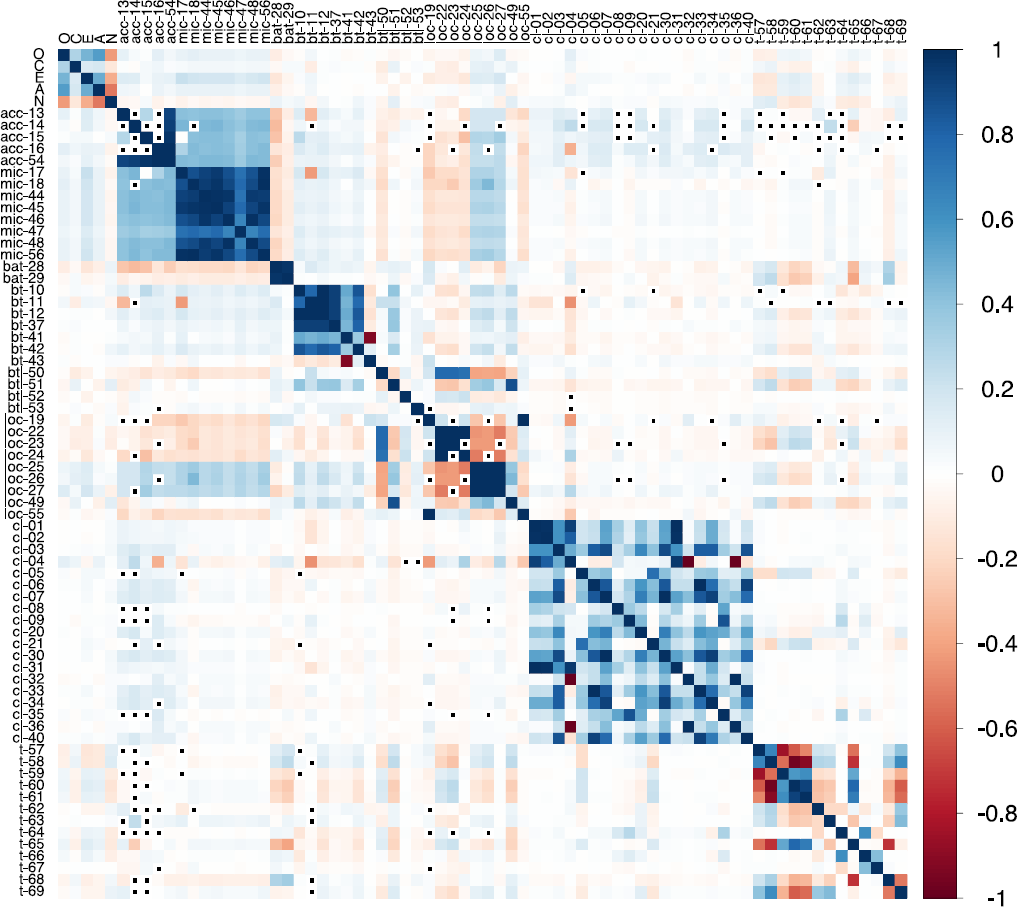
Plot of pairwise Spearman correlations. Note: · = correlation not available due to missing values. O = openness, C = conscientiousness, E = extraversion, A = agreeableness, N = neuroticism. ‘acc’ = accelerometer, ‘mic’ = microphone, ‘bat’ = battery, ‘bt’ = Bluetooth, ‘btl’ = Bluetooth & location, ‘loc’ = location, ‘cl’ = phone calls, ‘t’ = time. Numbers correspond to the ‘ID’ used in previous tables.
Further, there are many strong correlations (|ρ| > .90 for 50 variable pairs) among indicator variables that are based on the same data source. Especially, the set of microphone indicators and the set of Bluetooth indicators show large pairwise correlations among themselves. Pairwise correlations between indicators based on different data sources are generally small to moderate (mostly |ρ| < .20 and almost all |ρ| < .40), but clearly, the indicators from accelerometer and microphone are linked, with comparatively high positive correlations.
Overall, the correlation analysis shows only weak associations between smartphone data and ipsatized personality states and also demonstrates that there is some redundancy in the indicators, mostly among indicators from the same data source.
Step 2—Prediction analysis
In Figure 2, we show the results of applying fivefold nested cross–validation for estimating the prediction performance on out–of–sample data using the coefficient of determination (R2) measure. We used the formula for cross–validated R2 that was used in related work (Stachl et al., 2020). Because of the ipsatization, the R2 of the baseline model that learns and predicts the mean personality state level is always exactly zero and is therefore omitted from the figure. Table 8 additionally shows the prediction performance using mean absolute error and Pearson correlation. The results suggest that only for extraversion, prediction based on our smartphone data clearly and substantially surpassed prediction using only time–based indicators. Indeed, only for extraversion, the prediction performance was consistently better or equal across all cross–validation splits. As we have applied techniques for mitigating the problem of having too many predictor variables, this suggests that for openness, conscientiousness, agreeableness, and neuroticism, the current indicators based on smartphone data may not be informative beyond what can be inferred purely on the basis of time. However, even for extraversion, the mean R2 value is small (about 0.06), meaning that the variance captured by the model is only about 6%.
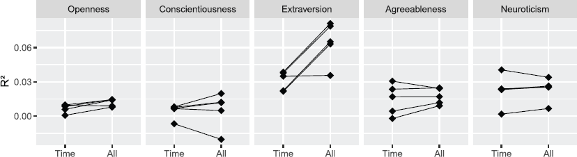
Prediction performance (R2) on the 5 cross–validation folds. Note: Data points are results from individual cross–validation folds. Lines connect identical folds.
Prediction performance (mean across five cross–validation folds)
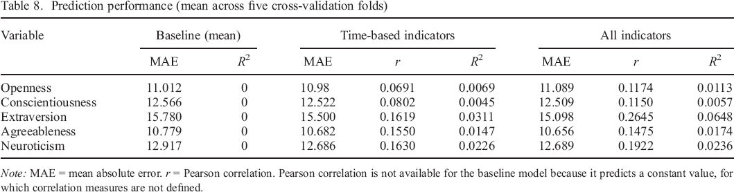
Note: MAE = mean absolute error. r = Pearson correlation. Pearson correlation is not available for the baseline model because it predicts a constant value, for which correlation measures are not defined.
Inspecting the models that were picked by the model selection on the full set of indicators, we observed that XGBoost (without SFFS) and Lasso regression were chosen for extraversion, for others, mostly Ridge and Lasso regression were chosen. PCA was never used in the selected models. Indicator set B was always chosen for extraversion, for the other dimensions, indicator set A was almost always preferred. Please see Appendix F for the list of all the selected models, as well as additional analyses.
Step 3—Analysis of multivariate associations
The results of the repeated feature selection using the best simple models on the bootstrapped samples are shown in Table 9. It contains the ranked lists of indicators that were most often selected by the feature selection process. We listed only the indicators that were selected at least 10 times, in order to focus on the more reliable indicators. If multiple models selected the same indicators, we listed only the simplest model in the table, that is, the one using the smallest indicator set, or the smallest number of selected features. Overall, with few exceptions, the selected indicators are all either based on microphone, time, or location. Notably, smartphone–data indicators were most often selected in all models for Openness, Conscientiousness, and Extraversion, suggesting that these smartphone–data indicators are relatively more predictive compared to all other indicators. Single smartphone–data indicators that were most often selected are ID–56 (Microphone dB), ID–49 (Time at work location), and to a lesser extent ID–22 (Time at home location).
Features selected by the feature selection process (all indicators)
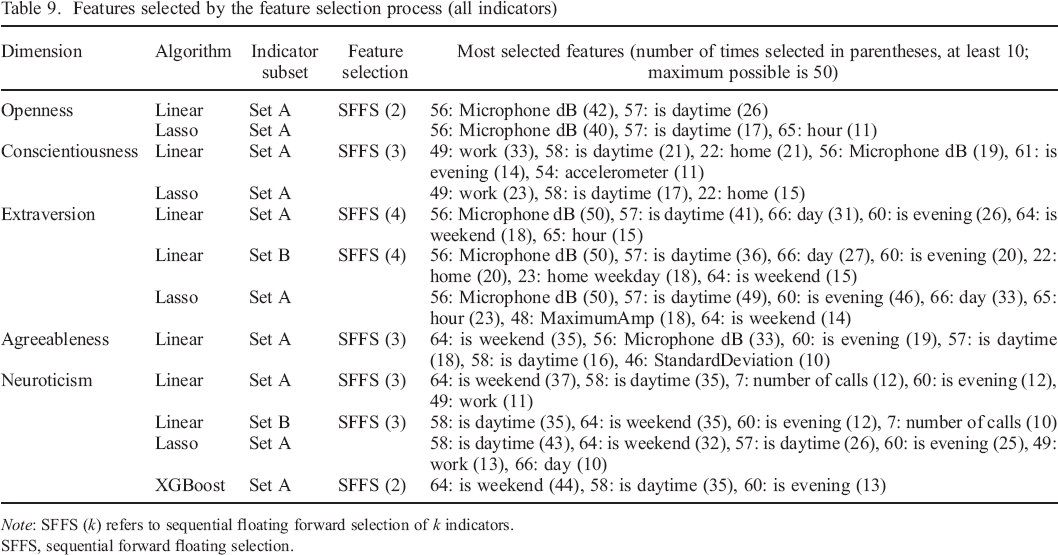
Note: SFFS (k) refers to sequential floating forward selection of k indicators.
SFFS, sequential forward floating selection.
Discussion
The goal of the current work was to explore the associations between Big Five personality states assessed on the past 30 minutes and smartphone data collected in the same time frame. To the best of our knowledge, this study is the first to investigate associations between Big Five personality states and smartphone data.
We developed behavioural and situational indicators from prior work and applied them on a new experience sampling data set. Our analysis of direct correlations among personality state levels and indicator values showed mostly small correlations between states and indicators, but highlighted associations among indicators of the same data source, principally between accelerometer and microphone indicators. Predictability of personality state levels was low. Only for extraversion, our evidence suggests a relationship between smartphone data and states that cannot be explained by the similarity of their temporal patterns. For other dimensions, this is not the case, as smartphone data were not informative beyond what could be predicted from the time and weekday of sampling alone. Overall, linear models appeared to be similarly predictive as models that can exploit non–linear associations and variable interactions, which suggests that the found associations are mostly linear and without interactions.
Our finding of state predictability mostly for extraversion echoes the results of Mønsted et al. (2018) about the prediction of Big Five traits: only trait extraversion could be predicted from smartphone data. This may be because extraversion is fundamentally a more observable trait, not only for other people (Vazire, 2010) but also for smartphones. An alternative explanation that has been proposed is that smartphones ‘by their nature are devices for inter–human communication’ (Mønsted et al., 2018). However, other studies have found other Big Five traits to be similarly predictable as extraversion. On the one hand, Stachl et al. (2020) applied a maximally broad variety of data sources, and their results suggest the relevance of specific data sources for predicting personality traits other than extraversion, especially app–usage data. This data source was not available in our data set. On the other hand, Wang et al. (2018) focused on patterns of variability and provided evidence that some Big Five dimensions may be revealed less through specific behaviours or situations that can be sensed over a short time period, but through patterns that can only be observed in the long–term. In particular, patterns of regularity in daily behaviours seem to be important for inferring the trait conscientiousness (Stachl et al., 2020).
Our data set included 5748 experience sampling responses, which is nearly double of what was analysed by Kalimeri et al. (2013). Nevertheless, we found fewer associations of personality states with our indicators and also lower predictability. The contrast is potentially even greater, considering that the number of participants in our study was almost six times as large, which may also increase predictability by making it more likely that patterns generalize between the sets of participants that are separated during cross–validation. This points to limitations of smartphones compared with specialized devices such as the sociometric badge. For example, the sociometric badge could record movement continuously at a high rate, instead of only sampling for 5 seconds every 5 minutes.
Our analysis showed that indicators based on measurements of loudness (from microphone) are predictive of extraversion state beyond what can be predicted from time–based indicators. This result seems rather intuitive: typical extravert behaviour includes being talkative, assertive, and sociable (John & Srivastava, 1999), which should make it likely that the phone would sense (voice) sounds more often and at higher intensity. Also, it may be that for our sample, louder environments are typically places where people socialize, such as a bar or restaurant.
We also found that situational factors derived from the time of sampling (e.g. whether it was daytime, evening, and on a weekend or not) were predictive of personality states. This result is consistent with Fleeson (2001), who found that states of all Big Five dimensions except neuroticism were correlated with the time of day. It is also in line with broad evidence for diurnal patterns of behaviour and affect (Golder & Macy, 2011; Harari et al., 2019; Servia–Rodriguez et al., 2017).
With regard to potential applications, this study has found little evidence for the potential of using smartphone data measures to (partially) substitute personality state survey measures. Nevertheless, the association between microphone indicators and extraversion state suggests that more sophisticated processing of audio recordings has potential applications in assessment of extraversion state. Our results furthermore suggest that using time–based indicators should also be considered when studying personality states.
Limitations and future directions
Smartphone data collection studies are in general subject to important limitations. Study participants may not always keep their smartphones close by, which can bias both the experience sampling and mobile sensing data collections. There are also technical factors that can affect the data collection, for example, changes in the operating systems as smartphone vendors release updated operating system versions. These are complex issues that require further study.
As intense data collection on smartphones is subject to several trade–offs, it should be noted that this analysis is based on a single data collection effort, which used one particular schedule, set of data sources, and set of processes for data collection. Different implementations may collect data that are more informative about personality states. Also, our sample with mostly young students and employees can be expected to express personality states in some idiosyncratic ways. Furthermore, we only examined data from users of Android phones, who may differ from users of alternatives, though there is evidence that differences are small (Götz, Stieger, & Reips, 2017). Overall, the observed weak associations between smartphone data and personality states suggest that approaches or data sources beyond what was covered in this study are necessary for smartphones to play a role in unobtrusive assessment of personality states. This may include non–technical solutions such as collecting larger samples and providing additional incentives to study participants for submitting more complete data. Without additional measures, many participants may simply keep location and Bluetooth sensing deactivated on their phone.
On the technical side, a relatively simple improvement would be to collect sensing data at shorter intervals, but only during the time covered by the experience sampling, as opposed to continuously over the whole day as in our study. This would allow the collection of higher resolution data within the timeframe described by the personality state measurements, without negatively impacting battery life. More involved but promising sensing approaches that have already been applied in related work include detection of speech (Wang & Marsella, 2017; Wang et al., 2018), analysis of speaking sounds (Kalimeri et al., 2013), and collecting additional data from personal computer use (Grover & Mark, 2017). Future research should also include data from increasingly common mobile devices such as smartwatches and conduct more sophisticated analysis of audio data, such as speaker identification and analysis of ambient noise (Lane, Georgiev, & Qendro, 2015). However, these improvements may not reduce current challenges with battery drain and privacy concerns but could actually exacerbate them.
Collecting additional data that contain more information about personality states, especially other than extraversion, will be highly relevant future work. As pointed out previously by Bleidorn, Hopwood, and Wright (2017), a large amount of future work will be needed for the development of interpretable and validated indicators that can be reliably used for behavioural assessment of personality states. The following considerations appear relevant for future work on mobile sensing state assessment with respect to the individual Big Five dimensions. State openness seems generally challenging to assess through mobile sensing, as what constitutes open behaviour may only be clear relative to a comprehensive assessment of a person's past behaviours. Similarly, what constitutes conscientious behaviour could depend on a person's goals and duties. As noted by Boyd, Pasca, and Lanning (2020), the contextual nature of behaviour may need to be given more attention when exploring links between behaviour and conceptions of personality. Based on conscientiousness’ negative association with distractibility, assessment of common distractive behaviours such as social media use may provide relatively universal indicators of low conscientiousness states (Mark, Czerwinski, & Iqbal, 2018). In general, app–usage data may be relevant for assessing most Big Five personality state dimensions, as it was found relevant for inferring all Big Five traits other than agreeableness (Stachl et al., 2020). Heart rate data from smartwatches or fitness trackers are likely useful for inferring state neuroticism and state agreeableness (specifically, anger), as heart rate variability is affected by the stress response (Kim, Cheon, Bai, Lee, & Koo, 2018).
The measures for assessing personality states that were used in our analysis should also be reconsidered. When relating measures of personality states to sensing data, the strength of relations with subjective measures will always be limited by subjective tendencies. Therefore, observer reports should also be explored, ideally by combining reports from multiple observers to compensate for each observer's subjective tendencies and possibly focusing on measures with higher observer agreement. For example, a study using smartphone data collection along with audio recordings that are observer–rated (as in Sun & Vazire, 2019) could be highly valuable. Based on consensual observer ratings, objective measures with high validity may be achievable for some behavioural elements of personality, such as talkativeness. Finally, it may be beneficial to update the conceptualizations of personality themselves, based on data that describes objective behaviours (Boyd et al., 2020).
Additional important relationships also remain to be explored. Trait levels may affect state levels beyond simple average values and may show complex interactions with situational variables, thus they should also be included in future analyses.
Publication of Data Set
The anonymized data set and the data analysis scripts are available at https://osf.io/j93bs/.
Sampling Statement
The sample size of the collected data was determined by the requirements of the PEACH study (Stieger et al., 2018). Because of our use of machine learning, we could not estimate the required number of samples by a traditional analysis of statistical power for the present work. Instead, we determined that the number of samples should not be lower than the number of samples analysed in the most similar previous work (Kalimeri et al., 2013). This criterion is fulfilled, because our number of study participants is almost six times as large, and the number of state samples is more than 80% larger than the number of samples analysed by Kalimeri et al. (2013). Because of the much larger number of study participants, our findings are likely to better generalize beyond the participant population.
Open Science Disclosure Statement
We confirm that we have reported all measures, conditions, data exclusions, and sample size determination strategies for this work, either in this article or in the published study protocol (Stieger et al., 2018).
Funding Information
Work on this manuscript was partially supported by a grant from the Swiss National Science Foundation (162724).
Ethics Approval
Data collection was consistent with ethical standards for the treatment of human subjects and approved by the Ethics Commission of the Philosophical Faculty of the University of Zurich, Switzerland (No. 17.8.4).
Supporting Information
Supporting Information, per2309-sup-0001 - How Are Personality States Associated with Smartphone Data?
Supporting info item
Supporting Information, per2309-sup-0001 for How Are Personality States Associated with Smartphone Data? by DOMINIK Rüegger, MIRJAM STIEGER, MARCIA Nißen, MATHIAS ALLEMAND, ELGAR FLEISCH and TOBIAS KOWATSCH, in European Journal of Personality
Supporting info item
Footnotes
Supporting Information
Additional supporting information may be found online in the Supporting Information section at the end of the article.
State Measurement
Figure A1 depicts the user interface for the assessment of the states. Figure A2 shows the histograms of the self–reported personality state values for each dimension, before ipsatization. The histograms for openness, conscientiousness, and agreeableness are similar, with most values in the upper half of the scale, whereas this is reversed for neuroticism, and for extraversion the values are more balanced.
Selection of Indicators from Stachl et AL.
As only few associations between Big Five traits and indicators from smartphone data were reported in the main paper, we analysed the supplied additional materials to determine the associations. As elastic net regression can shrink irrelevant coefficients to zero (Friedman et al., 2001), we considered all indicators as associated that had a non–zero standardized beta coefficient as reported in the files ‘EN_betacoef_std_*.csv’ in the folder ‘OSF–Repo/data/modeling/results/feature_importance/’, where ‘*’ stands for a Big Five dimension. With random forests, Stachl et al. (2020) also computed permutation importance (Altmann, Toloşi, Sander, & Lengauer, 2010), which is a measure of relevance for individual indicators. We considered all indicators as associated with feature importance larger than zero, as reported in the files ‘RF_featImpPermu_*.csv’ in the mentioned folder.
Implementation of Indicators
In order to facilitate the reproducibility of this work, we discuss some important aspects of the implementation of our indicators.
Indicator Distributions
Indicator statistics
| ID | Description | Zero (%) | Missing (%) | Other (%) | Mean | Median | Min | Max |
|---|---|---|---|---|---|---|---|---|
| 1 | Calls incoming | 68 | 30 | 1 | 0.024 | 0 | 0 | 3 |
| 2 | Time spent in incoming calls | 69 | 30 | 1 | 0.064 | 0 | 0 | 24.3 |
| 3 | Time spent in calls | 66 | 30 | 4 | 0.21 | 0 | 0 | 26.4 |
| 4 | Response rate | 1 | 98 | 1 | 0.61 | 1 | 0 | 1 |
| 5 | Call during night | 69 | 30 | 52 | 0.018 | 0 | 0 | 6 |
| 6 | Number of initiated calls | 66 | 30 | 4 | 0.073 | 0 | 0 | 5 |
| 7 | Number of calls | 65 | 30 | 5 | 0.11 | 0 | 0 | 6 |
| 8 | Calls InDayWknd | 70 | 30 | 10 | 0.0027 | 0 | 0 | 2 |
| 9 | Calls OutDayWknd | 70 | 30 | 27 | 0.0099 | 0 | 0 | 4 |
| 10 | Bt devices in the environment if daytime | 7 | 70 | 23 | 6 | 2 | 0 | 213 |
| 11 | Bt Devices in the environment if evening | 4 | 88 | 9 | 3.2 | 1 | 0 | 185 |
| 12 | Bt Devices in the environment | 10 | 58 | 32 | 5.2 | 2 | 0 | 213 |
| 13 | Accelerometer during commute | 0 | 79 | 21 | 0.47 | 0.14 | 0.0054 | 8.2 |
| 14 | Accelerometer during lunch | 0 | 84 | 16 | 0.48 | 0.22 | 0.0045 | 5.4 |
| 15 | Accelerometer during evening | 0 | 79 | 21 | 0.48 | 0.18 | 0.005 | 10.5 |
| 16 | Accelerometer during weekend | 0 | 87 | 13 | 0.45 | 0.15 | 0.0058 | 5.3 |
| 17 | Microphone commute or lunch | 0 | 66 | 34 | 58.5 | 59.7 | 5.9 | 88.3 |
| 18 | Microphone evening or weekend | 0 | 68 | 32 | 57.5 | 58.4 | 13.6 | 89.3 |
| 19 | Number of locations visited on weekend | 1 | 91 | 8 | 0.9 | 1 | 0 | 2 |
| 20 | Calls during commute lunch or weekends | 68 | 30 | 2 | 0.057 | 0 | 0 | 6 |
| 21 | Calls during evenings | 69 | 30 | 1 | 0.026 | 0 | 0 | 6 |
| 22 | Home time | 53 | 35 | 12 | 0.16 | 0 | 0 | 1 |
| 23 | Home time weekday | 42 | 50 | 8 | 0.14 | 0 | 0 | 1 |
| 24 | Home time weekend | 11 | 85 | 4 | 0.23 | 0 | 0 | 1 |
| 25 | Max distance home | 0 | 35 | 64 | 17.5 | 1.8 | 0 | 1146.5 |
| 26 | Max distance home weekday | 0 | 50 | 50 | 13.4 | 2 | 0 | 1146.5 |
| 27 | Max distance home weekend | 0 | 85 | 15 | 31.6 | 1.1 | 0 | 1146.4 |
| 28 | Mean charge connected | 0 | 84 | 16 | 62.2 | 66.9 | 0.33 | 100 |
| 29 | Mean charge disconnected | 0 | 11 | 89 | 59.8 | 62 | 0.96 | 100 |
| 30 | Number of call contacts | 65 | 30 | 5 | 0.091 | 0 | 0 | 5 |
| 31 | Number of call contacts incoming | 68 | 30 | 1 | 0.022 | 0 | 0 | 2 |
| 32 | Number of call contacts missed | 69 | 30 | 54 | 0.013 | 0 | 0 | 2 |
| 33 | Number of call contacts outgoing | 66 | 30 | 4 | 0.064 | 0 | 0 | 5 |
| 34 | Number of call contacts weekday | 66 | 30 | 4 | 0.081 | 0 | 0 | 5 |
| 35 | Number of call contacts weekend | 69 | 30 | 36 | 0.01 | 0 | 0 | 2 |
| 36 | Number of missed calls | 69 | 30 | 54 | 0.014 | 0 | 0 | 2 |
| 37 | Number of unique devices | 48 | 20 | 32 | 2.4 | 0 | 0 | 114 |
| 38 | Response rate calls others | 0 | 100 | 0 | — | — | — | — |
| 39 | Response rate calls user | 0 | 100 | 0 | — | — | — | — |
| 40 | Time spent in outgoing calls | 67 | 30 | 3 | 0.14 | 0 | 0 | 26.4 |
| 41 | PeopleCloseDist | 31 | 58 | 11 | 0.63 | 0 | 0 | 99 |
| 42 | PeopleInterDist | 17 | 58 | 24 | 2.8 | 0.66 | 0 | 184 |
| 43 | MeanDistance | 0 | 73 | 27 | 2.6 | 3 | 1 | 3 |
| 44 | MeanEnergy | 0 | 12 | 88 | 2.92E+07 | 2.62E+06 | 1.9 | 9.83E+08 |
| 45 | MeanAmplitude | 0 | 12 | 88 | 2479 | 1042.2 | 0.47 | 30 955.8 |
| 46 | StandardDeviation | 0 | 12 | 88 | 1587.2 | 833.8 | 0.85 | 11 653.3 |
| 47 | MinimumAmp | 2 | 12 | 86 | 219.9 | 51.5 | 0 | 6705 |
| 48 | MaximumAmp | 0 | 12 | 88 | 8505.1 | 4964.5 | 7 | 32 767 |
| 49 | Work time | 50 | 35 | 15 | 0.22 | 0 | 0 | 1 |
| 50 | Device count HOME | 38 | 56 | 6 | 0.3 | 0 | 0 | 28 |
| 51 | Device count WORK | 35 | 56 | 9 | 1.4 | 0 | 0 | 213 |
| 52 | Device count HOME OTHER | 43 | 56 | 24 | 0.013 | 0 | 0 | 3 |
| 53 | Device count OTHER WORK | 43 | 56 | 25 | 0.019 | 0 | 0 | 6.5 |
| 54 | Accelerometer | 0 | 6 | 94 | 0.46 | 0.17 | 1.11E–16 | 10.5 |
| 55 | Number of locations visited | 5 | 35 | 59 | 0.93 | 1 | 0 | 2 |
| 56 | Microphone dB | 0 | 12 | 88 | 57.5 | 58.5 | −6.3 | 89.8 |
| 57 | Is Daytime Golbeck | 15 | 3 | 82 | 0.84 | 1 | 0 | 1 |
| 58 | Is Daytime Wang | 29 | 3 | 68 | 0.7 | 1 | 0 | 1 |
| 59 | Is Evening Grover | 86 | 3 | 11 | 0.11 | 0 | 0 | 1 |
| 60 | Is Evening Wang | 69 | 3 | 28 | 0.28 | 0 | 0 | 1 |
| 61 | Is Evening Servia | 72 | 3 | 25 | 0.25 | 0 | 0 | 1 |
| 62 | Is Commute | 78 | 3 | 18 | 0.18 | 0 | 0 | 1 |
| 63 | Is Lunchtime | 83 | 3 | 14 | 0.14 | 0 | 0 | 1 |
| 64 | Is Weekend | 83 | 3 | 14 | 0.14 | 0 | 0 | 1 |
| 65 | Hour | 0 | 3 | 97 | 15.5 | 15.7 | 0.022 | 23.9 |
| 66 | Day | 16 | 3 | 81 | 2.4 | 2 | 0 | 6 |
| 67 | Is Friday | 81 | 3 | 16 | 0.16 | 0 | 0 | 1 |
| 68 | Is Morning | 74 | 3 | 22 | 0.23 | 0 | 0 | 1 |
| 69 | Is Afternoon | 51 | 3 | 46 | 0.47 | 0 | 0 | 1 |
Machine Learning Procedure
In total, we used three nested cross–validation procedures, as shown in Figure E1. The ‘inner loop’ was used by the SFFS algorithm to decide whether to add or remove an indicator to/from the selected set. We used the ‘middle loop’ for choosing k, the number of indicators that should be selected by the SFFS algorithm, as well as the parameters for ridge and lasso regressions, and PCA. Finally, the ‘outer loop’ was used to obtain a robust estimate of the prediction performance.
Importantly, we made sure to apply feature selection and PCA within each iteration of the outer cross–validation loop, instead of once on the complete data set. As has been pointed out by Friedman et al. (2001), selecting the features once on the complete set leads to an overestimation of the prediction accuracy on out–of–sample data, and the same applies to PCA. This is because selection of features and PCA provides exploitable information about patterns present in the portion of the data that are used for validation. As noted by Mønsted et al. (2018), this crucial aspect of the data analysis process may in fact have been ignored in previous work on prediction of personality traits from smartphone data, leading to exaggerated reports of predictability.
In Table E1, we provide an overview of the different modelling solutions that were compared within each “middle” loop. In total, we compared 42 different configurations.
Additional Results
In Tables F1 and F2, we listed the models that were selected in the models selection process for determining the best predictive performance among our candidate models. As we used five cross–validation folds, a maximum number of five models could be selected.
We also performed model selection to determine the best performance for each combination of feature set (time, or all indicators) and learning algorithm. Results are depicted in Figure F1. Differences appear small and may not be reliable.